Plotting with seaborn

ScmData provides limited support for plotting. However, we make it as easy as possible to return data in a format which can be used with the seaborn plotting library. Given the power of this library, we recommend having a look through its documentation if you want to make anything more than the most basic plots.

import matplotlib.pyplot as plt
import seaborn as sns

from scmdata.plotting import RCMIP_SCENARIO_COLOURS
from scmdata.run import ScmRun

/home/docs/checkouts/readthedocs.org/user_builds/scmdata/checkouts/stable/src/scmdata/database/_database.py:9: TqdmWarning: IProgress not found. Please update jupyter and ipywidgets. See https://ipywidgets.readthedocs.io/en/stable/user_install.html
  import tqdm.autonotebook as tqdman

Data

For this notebook we use the RCMIP radiative forcings, available at rcmip.org.

rcmip_db = ScmRun("rcmip-radiative-forcing-annual-means-v4-0-0.csv")
rcmip_db.head()

						time	1750-01-01 00:00:00	1751-01-01 00:00:00	1752-01-01 00:00:00	1753-01-01 00:00:00	1754-01-01 00:00:00	1755-01-01 00:00:00	1756-01-01 00:00:00	1757-01-01 00:00:00	1758-01-01 00:00:00	1759-01-01 00:00:00	...	2491-01-01 00:00:00	2492-01-01 00:00:00	2493-01-01 00:00:00	2494-01-01 00:00:00	2495-01-01 00:00:00	2496-01-01 00:00:00	2497-01-01 00:00:00	2498-01-01 00:00:00	2499-01-01 00:00:00	2500-01-01 00:00:00
activity_id	mip_era	model	region	scenario	unit	variable
not_applicable	CMIP5	AIM	World	rcp60	W/m^2	Radiative Forcing	NaN	NaN	NaN	NaN	NaN	NaN	NaN	NaN	NaN	NaN	...	5.993838	5.993838	5.993838	5.993838	5.993838	5.993838	5.993838	5.993838	5.993838	5.993838
						Radiative Forcing\|Anthropogenic	NaN	NaN	NaN	NaN	NaN	NaN	NaN	NaN	NaN	NaN	...	5.890082	5.890082	5.890082	5.890082	5.890082	5.890082	5.890082	5.890082	5.890082	5.890082
						Radiative Forcing\|Anthropogenic\|Aerosols	NaN	NaN	NaN	NaN	NaN	NaN	NaN	NaN	NaN	NaN	...	-0.603691	-0.603691	-0.603691	-0.603691	-0.603691	-0.603691	-0.603691	-0.603691	-0.603691	-0.603691
						Radiative Forcing\|Anthropogenic\|Aerosols\|Aerosols-cloud Interactions	NaN	NaN	NaN	NaN	NaN	NaN	NaN	NaN	NaN	NaN	...	-0.465404	-0.465404	-0.465404	-0.465404	-0.465404	-0.465404	-0.465404	-0.465404	-0.465404	-0.465404
						Radiative Forcing\|Anthropogenic\|Aerosols\|Aerosols-radiation Interactions	NaN	NaN	NaN	NaN	NaN	NaN	NaN	NaN	NaN	NaN	...	-0.138286	-0.138286	-0.138286	-0.138286	-0.138286	-0.138286	-0.138286	-0.138286	-0.138286	-0.138286

5 rows × 751 columns

Plotting with ScmRun

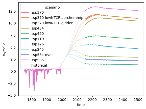
For the most common plotting patterns, we provide a very simple lineplot method in ScmRun.

out = rcmip_db.filter(variable="Effective Radiative Forcing").lineplot()
out

<Axes: xlabel='time', ylabel='W/m^2'>

../_images/2d30b9ff0e6db06782059292a105215594f6dd0ea578a2a712f366a76d859f4d.png

kwargs passed to this method are given directly to seaborn.lineplot, which allows an extra layer of control.

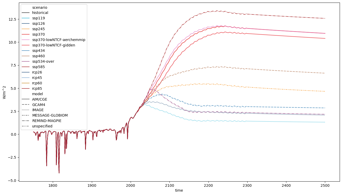
For example, we can plot on slightly bigger axes, make the lines slightly transparent, add markers for the different models, specify the colour to use for each scenario and specify the order to display the scenarios in.

ax = plt.figure(figsize=(16, 9)).add_subplot(111)
rcmip_db.filter(variable="Effective Radiative Forcing").lineplot(
    ax=ax,
    hue="scenario",
    palette=RCMIP_SCENARIO_COLOURS,
    hue_order=RCMIP_SCENARIO_COLOURS.keys(),
    style="model",
    alpha=0.7,
)

<Axes: xlabel='time', ylabel='W/m^2'>

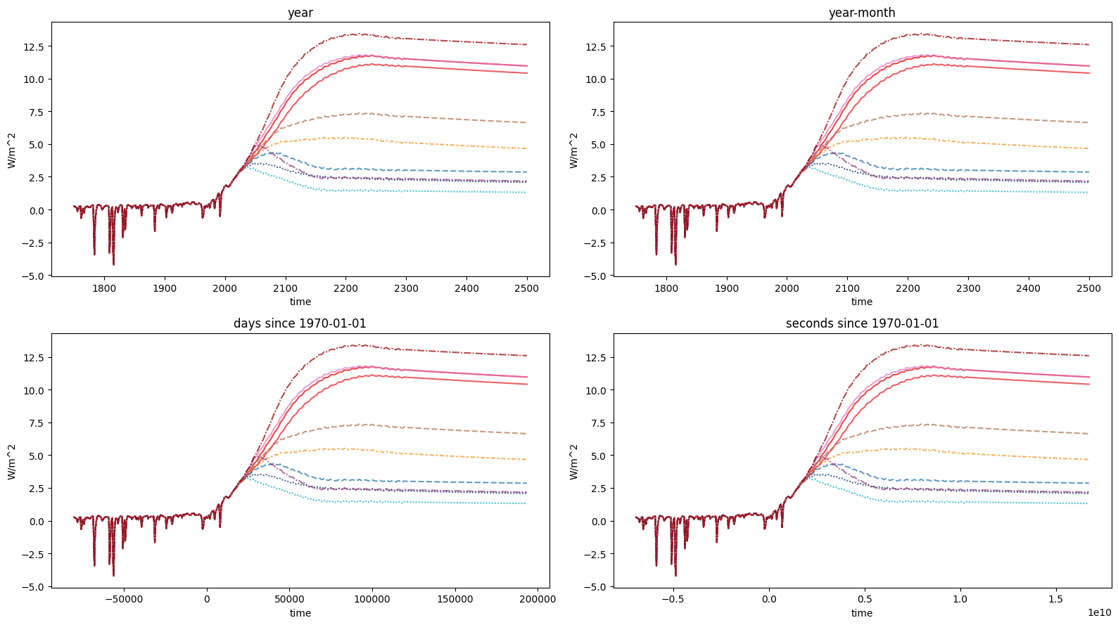
../_images/ba2533ffafa4c21665da080963a17fce7669baeeb63bb9f877eaaa8bc041cc39.png

Specifying the time axis

Plotting with a datetime.datetime time axis is not always convenient. To address this, we provide the time_axis keyword argument. The options are available in the lineplot docstring.

print(rcmip_db.lineplot.__doc__)

    Make a line plot via `seaborn's lineplot

    See seaborn documentation for a complete description of the kwargs
    <https://seaborn.pydata.org/generated/seaborn.lineplot.html>`_

    If only a single unit is present, it will be used as the y-axis label.
    The axis object is returned so this can be changed by the user if desired.

    Parameters
    ----------
    time_axis : {None, "year", "year-month", "days since 1970-01-01", "seconds since 1970-01-01"}
        Time axis to use for the plot.

        If ``None``, :class:`datetime.datetime` objects will be used.

        If ``"year"``, the year of each time point  will be used.

        If ``"year-month"``, the year plus (month - 0.5) / 12  will be used.

        If ``"days since 1970-01-01"``, the number of days since 1st Jan 1970 will be
        used (calculated using the :mod:`datetime` module).

        If ``"seconds since 1970-01-01"``, the number of seconds  since 1st Jan 1970 will
        be used (calculated using the :mod:`datetime` module).

    **kwargs
        Keyword arguments to be passed to ``seaborn.lineplot``. If none are passed,
        sensible defaults will be used.

    Returns
    -------
    :class:`matplotlib.axes._subplots.AxesSubplot`
        Output of call to ``seaborn.lineplot``
    

fig, axes = plt.subplots(figsize=(16, 9), nrows=2, ncols=2)

pdb = rcmip_db.filter(variable="Effective Radiative Forcing")
for ax, time_axis in zip(
    axes.flatten(),
    [
        "year",
        "year-month",
        "days since 1970-01-01",
        "seconds since 1970-01-01",
    ],
):
    pdb.lineplot(
        ax=ax,
        hue="scenario",
        palette=RCMIP_SCENARIO_COLOURS,
        hue_order=RCMIP_SCENARIO_COLOURS.keys(),
        style="model",
        alpha=0.7,
        time_axis=time_axis,
        legend=False,
    )
    ax.set_title(time_axis)

plt.tight_layout()

../_images/c36c2a5ab5476945bbbe343cb9d852ae143eefe2a4d0acd5f1142eca7f26bcf2.png

These same options can also be passed to the timeseries and long_data methods.

rcmip_db.timeseries(time_axis="year-month")

						time	1750.041667	1751.041667	1752.041667	1753.041667	1754.041667	1755.041667	1756.041667	1757.041667	1758.041667	1759.041667	...	2491.041667	2492.041667	2493.041667	2494.041667	2495.041667	2496.041667	2497.041667	2498.041667	2499.041667	2500.041667
activity_id	mip_era	model	region	scenario	unit	variable
not_applicable	CMIP5	AIM	World	rcp60	W/m^2	Radiative Forcing	NaN	NaN	NaN	NaN	NaN	NaN	NaN	NaN	NaN	NaN	...	5.993838	5.993838	5.993838	5.993838	5.993838	5.993838	5.993838	5.993838	5.993838	5.993838
						Radiative Forcing\|Anthropogenic	NaN	NaN	NaN	NaN	NaN	NaN	NaN	NaN	NaN	NaN	...	5.890082	5.890082	5.890082	5.890082	5.890082	5.890082	5.890082	5.890082	5.890082	5.890082
						Radiative Forcing\|Anthropogenic\|Aerosols	NaN	NaN	NaN	NaN	NaN	NaN	NaN	NaN	NaN	NaN	...	-0.603691	-0.603691	-0.603691	-0.603691	-0.603691	-0.603691	-0.603691	-0.603691	-0.603691	-0.603691
						Radiative Forcing\|Anthropogenic\|Aerosols\|Aerosols-cloud Interactions	NaN	NaN	NaN	NaN	NaN	NaN	NaN	NaN	NaN	NaN	...	-0.465404	-0.465404	-0.465404	-0.465404	-0.465404	-0.465404	-0.465404	-0.465404	-0.465404	-0.465404
						Radiative Forcing\|Anthropogenic\|Aerosols\|Aerosols-radiation Interactions	NaN	NaN	NaN	NaN	NaN	NaN	NaN	NaN	NaN	NaN	...	-0.138286	-0.138286	-0.138286	-0.138286	-0.138286	-0.138286	-0.138286	-0.138286	-0.138286	-0.138286
		...	...	...	...	...	...	...	...	...	...	...	...	...	...	...	...	...	...	...	...	...	...	...	...	...	...
		unspecified	World	historical-cmip5	W/m^2	Radiative Forcing\|Anthropogenic\|Stratospheric Ozone	NaN	NaN	NaN	NaN	NaN	NaN	NaN	NaN	NaN	NaN	...	NaN	NaN	NaN	NaN	NaN	NaN	NaN	NaN	NaN	NaN
						Radiative Forcing\|Anthropogenic\|Tropospheric Ozone	NaN	NaN	NaN	NaN	NaN	NaN	NaN	NaN	NaN	NaN	...	NaN	NaN	NaN	NaN	NaN	NaN	NaN	NaN	NaN	NaN
						Radiative Forcing\|Natural	NaN	NaN	NaN	NaN	NaN	NaN	NaN	NaN	NaN	NaN	...	NaN	NaN	NaN	NaN	NaN	NaN	NaN	NaN	NaN	NaN
						Radiative Forcing\|Natural\|Solar	NaN	NaN	NaN	NaN	NaN	NaN	NaN	NaN	NaN	NaN	...	NaN	NaN	NaN	NaN	NaN	NaN	NaN	NaN	NaN	NaN
						Radiative Forcing\|Natural\|Volcanic	NaN	NaN	NaN	NaN	NaN	NaN	NaN	NaN	NaN	NaN	...	NaN	NaN	NaN	NaN	NaN	NaN	NaN	NaN	NaN	NaN

499 rows × 751 columns

rcmip_db.long_data(time_axis="days since 1970-01-01")

	activity_id	mip_era	model	region	scenario	unit	variable	time	value
0	not_applicable	CMIP5	AIM	World	rcp60	W/m^2	Radiative Forcing	-74874	0.000000
1	not_applicable	CMIP5	AIM	World	rcp60	W/m^2	Radiative Forcing	-74509	0.126027
2	not_applicable	CMIP5	AIM	World	rcp60	W/m^2	Radiative Forcing	-74144	0.273031
3	not_applicable	CMIP5	AIM	World	rcp60	W/m^2	Radiative Forcing	-73779	0.278871
4	not_applicable	CMIP5	AIM	World	rcp60	W/m^2	Radiative Forcing	-73413	0.242045
...	...	...	...	...	...	...	...	...	...
332450	not_applicable	CMIP5	unspecified	World	historical-cmip5	W/m^2	Radiative Forcing\|Natural\|Volcanic	11323	0.232444
332451	not_applicable	CMIP5	unspecified	World	historical-cmip5	W/m^2	Radiative Forcing\|Natural\|Volcanic	11688	0.232444
332452	not_applicable	CMIP5	unspecified	World	historical-cmip5	W/m^2	Radiative Forcing\|Natural\|Volcanic	12053	0.232444
332453	not_applicable	CMIP5	unspecified	World	historical-cmip5	W/m^2	Radiative Forcing\|Natural\|Volcanic	12418	0.232444
332454	not_applicable	CMIP5	unspecified	World	historical-cmip5	W/m^2	Radiative Forcing\|Natural\|Volcanic	12784	0.184018

332455 rows × 9 columns

Plotting with seaborn

If you wish to make plots which are more complex than this most basic pattern, a combination of seaborn and pandas reshaping is your best bet.

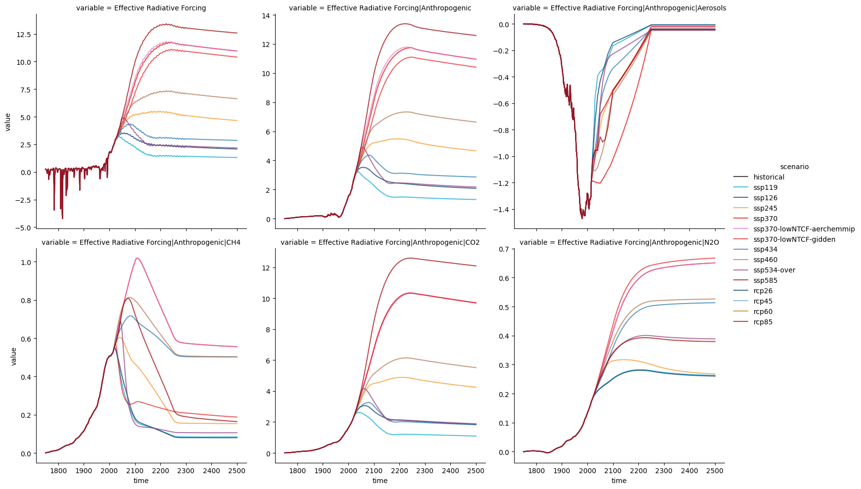
Plotting on a grid

Often we wish to look at lots of different variables at once. Seaborn allows this sort of ‘gridded’ plotting, as shown below.

vars_to_plot = ["Effective Radiative Forcing"] + [
    f"Effective Radiative Forcing|{v}"
    for v in [
        "Anthropogenic",
        "Anthropogenic|Aerosols",
        "Anthropogenic|CO2",
        "Anthropogenic|CH4",
        "Anthropogenic|N2O",
    ]
]
vars_to_plot

['Effective Radiative Forcing',
 'Effective Radiative Forcing|Anthropogenic',
 'Effective Radiative Forcing|Anthropogenic|Aerosols',
 'Effective Radiative Forcing|Anthropogenic|CO2',
 'Effective Radiative Forcing|Anthropogenic|CH4',
 'Effective Radiative Forcing|Anthropogenic|N2O']

seaborn_df = rcmip_db.filter(variable=vars_to_plot).long_data()
seaborn_df.head()

	activity_id	mip_era	model	region	scenario	unit	variable	time	value
0	not_applicable	CMIP6	AIM/CGE	World	ssp370	W/m^2	Effective Radiative Forcing	1750-01-01 00:00:00	0.259367
1	not_applicable	CMIP6	AIM/CGE	World	ssp370	W/m^2	Effective Radiative Forcing	1751-01-01 00:00:00	0.242788
2	not_applicable	CMIP6	AIM/CGE	World	ssp370	W/m^2	Effective Radiative Forcing	1752-01-01 00:00:00	0.214656
3	not_applicable	CMIP6	AIM/CGE	World	ssp370	W/m^2	Effective Radiative Forcing	1753-01-01 00:00:00	0.179488
4	not_applicable	CMIP6	AIM/CGE	World	ssp370	W/m^2	Effective Radiative Forcing	1754-01-01 00:00:00	0.145354

With the output of .long_data() we can directly use seaborn.relplot.

sns.relplot(
    data=seaborn_df,
    x="time",
    y="value",
    col="variable",
    col_wrap=3,
    hue="scenario",
    palette=RCMIP_SCENARIO_COLOURS,
    hue_order=RCMIP_SCENARIO_COLOURS.keys(),
    alpha=0.7,
    facet_kws={"sharey": False},
    kind="line",
)

<seaborn.axisgrid.FacetGrid at 0x7fc693c42ca0>

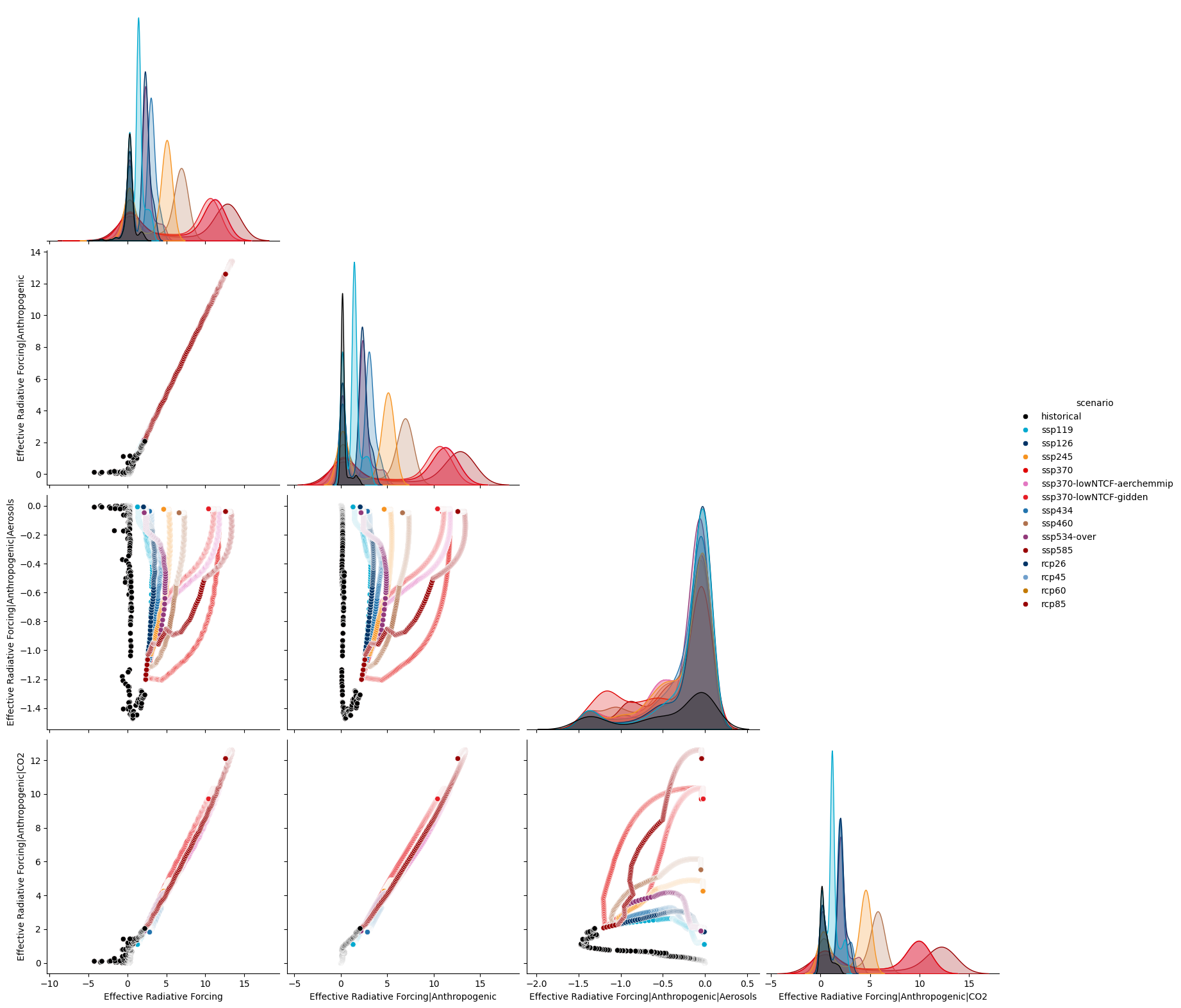
../_images/c30a7e6c05588930349ccd1c0e2a4232b9fd5b4311fc4404196a0ff64b68559f.png

Variable scatter plots

Sometimes we don’t want to plot against time, rather we want to plot variables against each other. For example, we might want to see how the effective radiative forcings relate to each other in the different scenarios. In such a case we can reshape the data using pandas before using seaborn.

ts = rcmip_db.filter(variable=vars_to_plot[:4]).timeseries()
ts.head()

						time	1750-01-01 00:00:00	1751-01-01 00:00:00	1752-01-01 00:00:00	1753-01-01 00:00:00	1754-01-01 00:00:00	1755-01-01 00:00:00	1756-01-01 00:00:00	1757-01-01 00:00:00	1758-01-01 00:00:00	1759-01-01 00:00:00	...	2491-01-01 00:00:00	2492-01-01 00:00:00	2493-01-01 00:00:00	2494-01-01 00:00:00	2495-01-01 00:00:00	2496-01-01 00:00:00	2497-01-01 00:00:00	2498-01-01 00:00:00	2499-01-01 00:00:00	2500-01-01 00:00:00
activity_id	mip_era	model	region	scenario	unit	variable
not_applicable	CMIP6	AIM/CGE	World	ssp370	W/m^2	Effective Radiative Forcing	0.259367	0.242788	0.214656	0.179488	0.145354	0.098651	-0.133032	0.016012	0.147192	0.226591	...	10.978680	10.976215	10.973747	10.971275	10.968806	10.966383	10.963918	10.961447	10.959022	10.957785
						Effective Radiative Forcing\|Anthropogenic	0.000000	0.001756	0.003698	0.004707	0.004987	0.007033	0.008562	0.008844	0.010441	0.011487	...	10.978680	10.976215	10.973747	10.971275	10.968806	10.966383	10.963918	10.961447	10.959022	10.957785
						Effective Radiative Forcing\|Anthropogenic\|Aerosols	0.000000	0.000836	0.001212	0.000801	-0.000571	0.000063	0.000618	-0.001421	-0.000764	-0.000720	...	-0.043755	-0.043755	-0.043755	-0.043755	-0.043755	-0.043755	-0.043755	-0.043755	-0.043755	-0.043755
						Effective Radiative Forcing\|Anthropogenic\|CO2	0.000000	0.000824	0.001647	0.002330	0.003153	0.004097	0.004859	0.005923	0.006866	0.007890	...	9.719260	9.716890	9.714518	9.712146	9.709772	9.707446	9.705070	9.702694	9.700365	9.699176
				ssp370-lowNTCF-aerchemmip	W/m^2	Effective Radiative Forcing	0.259367	0.242788	0.214656	0.179488	0.145354	0.098651	-0.133032	0.016012	0.147192	0.226591	...	10.969436	10.966971	10.964503	10.962031	10.959561	10.957139	10.954674	10.952202	10.949777	10.948541

5 rows × 751 columns

ts_reshaped = ts.unstack("variable").stack("time").reset_index()
ts_reshaped.head()

/tmp/ipykernel_809/4198992639.py:1: FutureWarning: The previous implementation of stack is deprecated and will be removed in a future version of pandas. See the What's New notes for pandas 2.1.0 for details. Specify future_stack=True to adopt the new implementation and silence this warning.
  ts_reshaped = ts.unstack("variable").stack("time").reset_index()

variable	activity_id	mip_era	model	region	scenario	unit	time	Effective Radiative Forcing	Effective Radiative Forcing\|Anthropogenic	Effective Radiative Forcing\|Anthropogenic\|Aerosols	Effective Radiative Forcing\|Anthropogenic\|CO2
0	not_applicable	CMIP6	AIM/CGE	World	ssp370	W/m^2	1750-01-01 00:00:00	0.259367	0.000000	0.000000	0.000000
1	not_applicable	CMIP6	AIM/CGE	World	ssp370	W/m^2	1751-01-01 00:00:00	0.242788	0.001756	0.000836	0.000824
2	not_applicable	CMIP6	AIM/CGE	World	ssp370	W/m^2	1752-01-01 00:00:00	0.214656	0.003698	0.001212	0.001647
3	not_applicable	CMIP6	AIM/CGE	World	ssp370	W/m^2	1753-01-01 00:00:00	0.179488	0.004707	0.000801	0.002330
4	not_applicable	CMIP6	AIM/CGE	World	ssp370	W/m^2	1754-01-01 00:00:00	0.145354	0.004987	-0.000571	0.003153

sns.pairplot(
    ts_reshaped,
    hue="scenario",
    palette=RCMIP_SCENARIO_COLOURS,
    hue_order=RCMIP_SCENARIO_COLOURS.keys(),
    corner=True,
    height=4,
)

<seaborn.axisgrid.PairGrid at 0x7fc692d7eee0>

../_images/0202855c6c29687e21124fd8e054bc45f74ca163e044d789409cb48a91b17a43.png