Processing
scmdata has some support for processing ScmRun instances to calculate statistics
of interest. Here we provide examples of how to use them.
At present, we can calculate:
crossing times (e.g. 1.5C crossing times)
crossing time quantiles
exceedance probabilities
peak
peak year
categorisation in line with SR1.5
a set of summary variables
Load some data
For this demonstration, we are going to use MAGICC output from [RCMIP Phase 2] as available at https://zenodo.org/record/4624566/files/data-processed-submission-database-hadcrut5-target-MAGICCv7.5.1.tar.gz?download=1. Here we have just extracted the air temperature output for the SSPs from 1995 to 2100.
import matplotlib.pyplot as plt
import numpy as np
import pandas as pd
import seaborn as sns

import scmdata.processing
from scmdata import ScmRun
/tmp/ipykernel_836/579853008.py:3: DeprecationWarning:
Pyarrow will become a required dependency of pandas in the next major release of pandas (pandas 3.0),
(to allow more performant data types, such as the Arrow string type, and better interoperability with other libraries)
but was not found to be installed on your system.
If this would cause problems for you,
please provide us feedback at https://github.com/pandas-dev/pandas/issues/54466

  import pandas as pd
/home/docs/checkouts/readthedocs.org/user_builds/scmdata/checkouts/stable/src/scmdata/database/_database.py:9: TqdmWarning: IProgress not found. Please update jupyter and ipywidgets. See https://ipywidgets.readthedocs.io/en/stable/user_install.html
  import tqdm.autonotebook as tqdman
magicc_output = ScmRun("magicc-rcmip-phase-2-gsat-output.csv")
magicc_output
<ScmRun (timeseries: 4800, timepoints: 106)>
Time:
	Start: 1995-01-01T00:00:00
	End: 2100-01-01T00:00:00
Meta:
	     climate_model  ensemble_member        model region scenario unit  \
	0     MAGICCv7.5.1                0  unspecified  World   ssp585    K
	1     MAGICCv7.5.1                1  unspecified  World   ssp585    K
	2     MAGICCv7.5.1                2  unspecified  World   ssp585    K
	3     MAGICCv7.5.1                3  unspecified  World   ssp585    K
	4     MAGICCv7.5.1                4  unspecified  World   ssp585    K
	...            ...              ...          ...    ...      ...  ...
	4795  MAGICCv7.5.1              595  unspecified  World   ssp119    K
	4796  MAGICCv7.5.1              596  unspecified  World   ssp119    K
	4797  MAGICCv7.5.1              597  unspecified  World   ssp119    K
	4798  MAGICCv7.5.1              598  unspecified  World   ssp119    K
	4799  MAGICCv7.5.1              599  unspecified  World   ssp119    K

	                            variable
	0     Surface Air Temperature Change
	1     Surface Air Temperature Change
	2     Surface Air Temperature Change
	3     Surface Air Temperature Change
	4     Surface Air Temperature Change
	...                              ...
	4795  Surface Air Temperature Change
	4796  Surface Air Temperature Change
	4797  Surface Air Temperature Change
	4798  Surface Air Temperature Change
	4799  Surface Air Temperature Change

	[4800 rows x 7 columns]
Crossing times
The first thing we do is show how to calculate the crossing times of a given threshold.
crossing_time_15 = scmdata.processing.calculate_crossing_times(
    magicc_output,
    threshold=1.5,
)
crossing_time_15
climate_model  ensemble_member  model        region  scenario  unit  variable
MAGICCv7.5.1   0                unspecified  World   ssp585    K     Surface Air Temperature Change    2025.0
               1                unspecified  World   ssp585    K     Surface Air Temperature Change    2029.0
               2                unspecified  World   ssp585    K     Surface Air Temperature Change    2024.0
               3                unspecified  World   ssp585    K     Surface Air Temperature Change    2023.0
               4                unspecified  World   ssp585    K     Surface Air Temperature Change    2023.0
                                                                                                        ...
               595              unspecified  World   ssp119    K     Surface Air Temperature Change    2023.0
               596              unspecified  World   ssp119    K     Surface Air Temperature Change       NaN
               597              unspecified  World   ssp119    K     Surface Air Temperature Change    2026.0
               598              unspecified  World   ssp119    K     Surface Air Temperature Change    2019.0
               599              unspecified  World   ssp119    K     Surface Air Temperature Change    2024.0
Length: 4800, dtype: float64
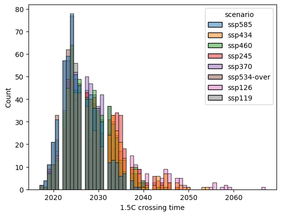
The output is a pd.Series, which is useful for many other pieces of work.
For example, we could make a plot with e.g. seaborn.
label = "1.5C crossing time"
pdf = crossing_time_15.reset_index().rename({0: label}, axis="columns")
sns.histplot(data=pdf, x=label, hue="scenario")
<Axes: xlabel='1.5C crossing time', ylabel='Count'>
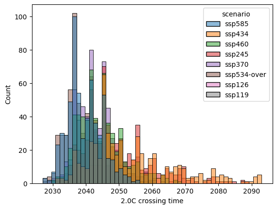
label = "2.0C crossing time"
crossing_time_20 = scmdata.processing.calculate_crossing_times(
    magicc_output,
    threshold=2.0,
)

pdf = crossing_time_20.reset_index().rename({0: label}, axis="columns")
sns.histplot(data=pdf, x=label, hue="scenario")
<Axes: xlabel='2.0C crossing time', ylabel='Count'>
Crossing time quantiles
Calculating the quantiles of crossing times is a bit fiddly because some ensemble members will not cross the threshold at all. We show how quantiles can be calculated sensibly below. The calculation will return nan if that quantile in the crossing times corresponds to an ensemble member which never crosses the threshold.
scmdata.processing.calculate_crossing_times_quantiles(
    crossing_time_15,
    groupby=["climate_model", "model", "scenario"],
    quantiles=(0.05, 0.17, 0.5, 0.83, 0.95),
)
climate_model  model        scenario     quantile
MAGICCv7.5.1   unspecified  ssp119       0.05        2021.00
                                         0.17        2023.00
                                         0.50        2027.00
                                         0.83            NaN
                                         0.95            NaN
                            ssp126       0.05        2021.00
                                         0.17        2023.00
                                         0.50        2028.00
                                         0.83        2038.17
                                         0.95            NaN
                            ssp245       0.05        2021.00
                                         0.17        2023.00
                                         0.50        2028.00
                                         0.83        2034.00
                                         0.95        2039.00
                            ssp370       0.05        2021.00
                                         0.17        2024.00
                                         0.50        2028.00
                                         0.83        2032.00
                                         0.95        2036.00
                            ssp434       0.05        2021.00
                                         0.17        2023.00
                                         0.50        2027.00
                                         0.83        2034.00
                                         0.95        2041.00
                            ssp460       0.05        2021.00
                                         0.17        2023.00
                                         0.50        2027.00
                                         0.83        2032.00
                                         0.95        2036.00
                            ssp534-over  0.05        2020.00
                                         0.17        2022.00
                                         0.50        2025.00
                                         0.83        2030.00
                                         0.95        2033.05
                            ssp585       0.05        2020.00
                                         0.17        2022.00
                                         0.50        2025.00
                                         0.83        2030.00
                                         0.95        2034.00
dtype: float64
In the above, we can see that the 83rd percentile of crossing times is in fact to not cross at all under the SSP1-1.9 scenario.
Datetime output
If desired, data could be interpolated first before calculating the crossing times. In such cases, returning the output as datetime rather than year might be helpful.
scmdata.processing.calculate_crossing_times(
    magicc_output.resample("MS"),
    threshold=2.0,
    return_year=False,
)
climate_model  ensemble_member  model        region  scenario  unit  variable
MAGICCv7.5.1   0                unspecified  World   ssp585    K     Surface Air Temperature Change   2042-02-01
               1                unspecified  World   ssp585    K     Surface Air Temperature Change   2041-10-01
               2                unspecified  World   ssp585    K     Surface Air Temperature Change   2035-11-01
               3                unspecified  World   ssp585    K     Surface Air Temperature Change   2035-09-01
               4                unspecified  World   ssp585    K     Surface Air Temperature Change   2036-01-01
                                                                                                         ...
               595              unspecified  World   ssp119    K     Surface Air Temperature Change          NaT
               596              unspecified  World   ssp119    K     Surface Air Temperature Change          NaT
               597              unspecified  World   ssp119    K     Surface Air Temperature Change          NaT
               598              unspecified  World   ssp119    K     Surface Air Temperature Change   2027-07-01
               599              unspecified  World   ssp119    K     Surface Air Temperature Change          NaT
Length: 4800, dtype: datetime64[ns]
Exceedance probabilities
Next we show how to calculate exceedance probabilities.
exceedance_probability_2C = scmdata.processing.calculate_exceedance_probabilities(
    magicc_output,
    process_over_cols=["ensemble_member", "variable"],
    threshold=2.0,
)
exceedance_probability_2C
climate_model  model        region  scenario     unit
MAGICCv7.5.1   unspecified  World   ssp119       dimensionless    0.091667
                                    ssp126       dimensionless    0.350000
                                    ssp245       dimensionless    0.995000
                                    ssp370       dimensionless    1.000000
                                    ssp434       dimensionless    0.868333
                                    ssp460       dimensionless    1.000000
                                    ssp534-over  dimensionless    0.983333
                                    ssp585       dimensionless    1.000000
Name: 2.0 exceedance probability, dtype: float64
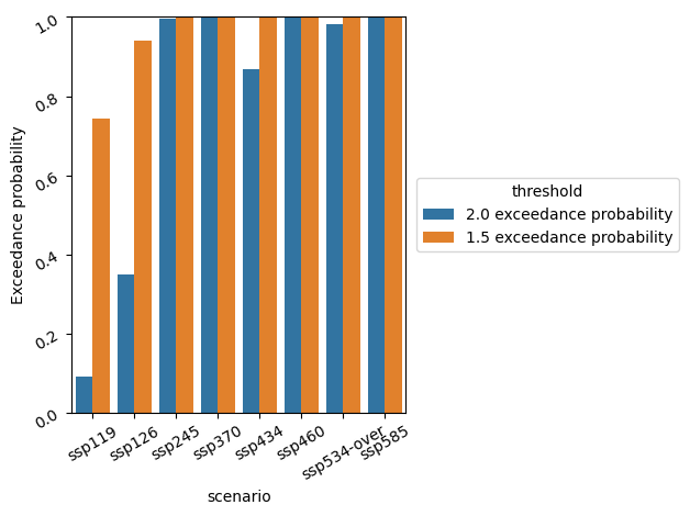
We can make a plot to compare exceedance probabilities over multiple scenarios.
exceedance_probability_15C = scmdata.processing.calculate_exceedance_probabilities(
    magicc_output,
    process_over_cols=["ensemble_member", "variable"],
    threshold=1.5,
)

pdf = (
    pd.DataFrame(
        [
            exceedance_probability_2C,
            exceedance_probability_15C,
        ]
    )
    .T.melt(ignore_index=False, value_name="Exceedance probability")
    .reset_index()
)
display(pdf)  # noqa

ax = sns.barplot(data=pdf, x="scenario", y="Exceedance probability", hue="variable")
ax.tick_params(labelrotation=30)
ax.set_ylim([0, 1])
ax.legend(loc="center left", bbox_to_anchor=(1.01, 0.5), title="threshold")
plt.tight_layout()
| climate_model | model | region | scenario | unit | variable | Exceedance probability | |
|---|---|---|---|---|---|---|---|
| 0 | MAGICCv7.5.1 | unspecified | World | ssp119 | dimensionless | 2.0 exceedance probability | 0.091667 |
| 1 | MAGICCv7.5.1 | unspecified | World | ssp126 | dimensionless | 2.0 exceedance probability | 0.350000 |
| 2 | MAGICCv7.5.1 | unspecified | World | ssp245 | dimensionless | 2.0 exceedance probability | 0.995000 |
| 3 | MAGICCv7.5.1 | unspecified | World | ssp370 | dimensionless | 2.0 exceedance probability | 1.000000 |
| 4 | MAGICCv7.5.1 | unspecified | World | ssp434 | dimensionless | 2.0 exceedance probability | 0.868333 |
| 5 | MAGICCv7.5.1 | unspecified | World | ssp460 | dimensionless | 2.0 exceedance probability | 1.000000 |
| 6 | MAGICCv7.5.1 | unspecified | World | ssp534-over | dimensionless | 2.0 exceedance probability | 0.983333 |
| 7 | MAGICCv7.5.1 | unspecified | World | ssp585 | dimensionless | 2.0 exceedance probability | 1.000000 |
| 8 | MAGICCv7.5.1 | unspecified | World | ssp119 | dimensionless | 1.5 exceedance probability | 0.743333 |
| 9 | MAGICCv7.5.1 | unspecified | World | ssp126 | dimensionless | 1.5 exceedance probability | 0.940000 |
| 10 | MAGICCv7.5.1 | unspecified | World | ssp245 | dimensionless | 1.5 exceedance probability | 1.000000 |
| 11 | MAGICCv7.5.1 | unspecified | World | ssp370 | dimensionless | 1.5 exceedance probability | 1.000000 |
| 12 | MAGICCv7.5.1 | unspecified | World | ssp434 | dimensionless | 1.5 exceedance probability | 1.000000 |
| 13 | MAGICCv7.5.1 | unspecified | World | ssp460 | dimensionless | 1.5 exceedance probability | 1.000000 |
| 14 | MAGICCv7.5.1 | unspecified | World | ssp534-over | dimensionless | 1.5 exceedance probability | 1.000000 |
| 15 | MAGICCv7.5.1 | unspecified | World | ssp585 | dimensionless | 1.5 exceedance probability | 1.000000 |
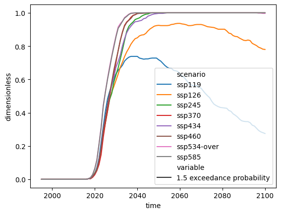
Exceedance probabilities over time
It is also possible to calculate exceedance probabilities over time.
res = scmdata.processing.calculate_exceedance_probabilities_over_time(
    magicc_output,
    process_over_cols="ensemble_member",
    threshold=1.5,
)
res = scmdata.ScmRun(res)
res.lineplot(style="variable")
<Axes: xlabel='time', ylabel='dimensionless'>
Note that taking the maximum exceedance probability over all time will be less
than or equal to the exceedance probability calculated with
calculate_exceedance_probabilities because the order of operations matters:
calculating whether each ensemble member exceeds the threshold or not then
seeing how many ensemble members out of the total exceed the threshold is not
the same as seeing how many ensemble members exceed the threshold at each
timestep and then taking the maximum over all timesteps. In general, taking
the maximum value from calculate_exceedance_probabilities_over_time will be
less than or equal to the results of calculate_exceedance_probabilities,
as demonstrated below.
comparison = (
    pd.DataFrame(
        {
            "calculate_exceedance_probabilities": exceedance_probability_15C,
            "max of calculate_exceedance_probabilities_over_time": (
                res.timeseries(meta=exceedance_probability_15C.index.names).max(axis=1)
            ),
        }
    )
    * 100
)
comparison.round(1)
| calculate_exceedance_probabilities | max of calculate_exceedance_probabilities_over_time | |||||
|---|---|---|---|---|---|---|
| climate_model | model | region | scenario | unit | ||
| MAGICCv7.5.1 | unspecified | World | ssp119 | dimensionless | 74.3 | 73.8 |
| ssp126 | dimensionless | 94.0 | 93.7 | |||
| ssp245 | dimensionless | 100.0 | 100.0 | |||
| ssp370 | dimensionless | 100.0 | 100.0 | |||
| ssp434 | dimensionless | 100.0 | 100.0 | |||
| ssp460 | dimensionless | 100.0 | 100.0 | |||
| ssp534-over | dimensionless | 100.0 | 100.0 | |||
| ssp585 | dimensionless | 100.0 | 100.0 |
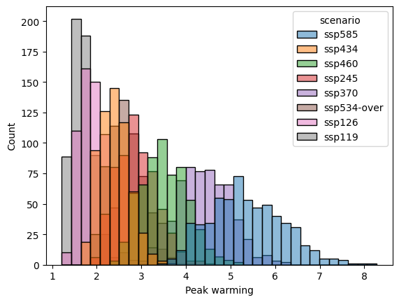
Peak
We can calculate the peaks in each timeseries.
peak_warming = scmdata.processing.calculate_peak(magicc_output)
peak_warming
climate_model  ensemble_member  model        region  scenario  unit  variable
MAGICCv7.5.1   0                unspecified  World   ssp585    K     Peak Surface Air Temperature Change    4.448044
               1                unspecified  World   ssp585    K     Peak Surface Air Temperature Change    5.372057
               2                unspecified  World   ssp585    K     Peak Surface Air Temperature Change    5.942238
               3                unspecified  World   ssp585    K     Peak Surface Air Temperature Change    5.220904
               4                unspecified  World   ssp585    K     Peak Surface Air Temperature Change    5.637467
                                                                                                              ...
               595              unspecified  World   ssp119    K     Peak Surface Air Temperature Change    1.809161
               596              unspecified  World   ssp119    K     Peak Surface Air Temperature Change    1.288471
               597              unspecified  World   ssp119    K     Peak Surface Air Temperature Change    1.669414
               598              unspecified  World   ssp119    K     Peak Surface Air Temperature Change    2.459078
               599              unspecified  World   ssp119    K     Peak Surface Air Temperature Change    1.746321
Name: 0, Length: 4800, dtype: float64
From this we can then calculate median peak warming by scenario (or other quantiles).
peak_warming.groupby(["model", "scenario"]).median()
model        scenario
unspecified  ssp119         1.653154
             ssp126         1.878890
             ssp245         2.838238
             ssp370         4.372581
             ssp434         2.371833
             ssp460         3.485626
             ssp534-over    2.613975
             ssp585         5.278692
Name: 0, dtype: float64
Or make a plot.
label = "Peak warming"
pdf = peak_warming.reset_index().rename({0: label}, axis="columns")
sns.histplot(data=pdf, x=label, hue="scenario")
<Axes: xlabel='Peak warming', ylabel='Count'>
Similarly to exceedance probabilties, the order of operations matters: calculating the median of the peaks is different to calculating the median then taking the peak of this median timeseries. In general, the max of the median timeseries is less than or equal to the median of the peak in each timeseries.
comparison = pd.DataFrame(
    {
        "median of peak warming": peak_warming.groupby(["model", "scenario"]).median(),
        "max of median timeseries": (
            magicc_output.process_over(
                list(set(magicc_output.meta.columns) - {"model", "scenario"}),
                "median",
            ).max(axis=1)
        ),
    }
)
comparison.round(3)
| median of peak warming | max of median timeseries | ||
|---|---|---|---|
| model | scenario | ||
| unspecified | ssp119 | 1.653 | 1.645 |
| ssp126 | 1.879 | 1.874 | |
| ssp245 | 2.838 | 2.838 | |
| ssp370 | 4.373 | 4.373 | |
| ssp434 | 2.372 | 2.368 | |
| ssp460 | 3.486 | 3.486 | |
| ssp534-over | 2.614 | 2.613 | |
| ssp585 | 5.279 | 5.279 |
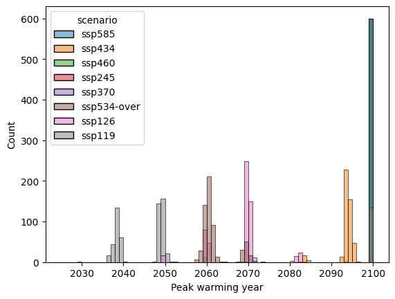
Peak time
We can calculate the peak time in each timeseries.
peak_warming_year = scmdata.processing.calculate_peak_time(magicc_output)
peak_warming_year
climate_model  ensemble_member  model        region  scenario  unit  variable
MAGICCv7.5.1   0                unspecified  World   ssp585    K     Year of peak Surface Air Temperature Change    2100
               1                unspecified  World   ssp585    K     Year of peak Surface Air Temperature Change    2100
               2                unspecified  World   ssp585    K     Year of peak Surface Air Temperature Change    2100
               3                unspecified  World   ssp585    K     Year of peak Surface Air Temperature Change    2100
               4                unspecified  World   ssp585    K     Year of peak Surface Air Temperature Change    2100
                                                                                                                    ...
               595              unspecified  World   ssp119    K     Year of peak Surface Air Temperature Change    2048
               596              unspecified  World   ssp119    K     Year of peak Surface Air Temperature Change    2036
               597              unspecified  World   ssp119    K     Year of peak Surface Air Temperature Change    2039
               598              unspecified  World   ssp119    K     Year of peak Surface Air Temperature Change    2059
               599              unspecified  World   ssp119    K     Year of peak Surface Air Temperature Change    2048
Name: 0, Length: 4800, dtype: int64
From this we can then calculate median peak warming time by scenario (or other quantiles).
peak_warming_year.groupby(["model", "scenario"]).median()
model        scenario
unspecified  ssp119         2048.0
             ssp126         2069.0
             ssp245         2100.0
             ssp370         2100.0
             ssp434         2094.0
             ssp460         2100.0
             ssp534-over    2060.0
             ssp585         2100.0
Name: 0, dtype: float64
label = "Peak warming year"
pdf = peak_warming_year.reset_index().rename({0: label}, axis="columns")
ax = sns.histplot(data=pdf, x=label, hue="scenario", bins=np.arange(2025, 2100 + 1))
SR1.5 categorisation
It is also possible to categorise the scenarios using the same categorisation as in SR1.5. To do this we have to first calculate the appropriate quantiles.
magicc_output_categorisation_quantiles = scmdata.ScmRun(
    magicc_output.quantiles_over("ensemble_member", quantiles=[0.33, 0.5, 0.66])
)
magicc_output_categorisation_quantiles
/home/docs/checkouts/readthedocs.org/user_builds/scmdata/checkouts/stable/src/scmdata/run.py:197: PerformanceWarning: DataFrame is highly fragmented.  This is usually the result of calling `frame.insert` many times, which has poor performance.  Consider joining all columns at once using pd.concat(axis=1) instead. To get a de-fragmented frame, use `newframe = frame.copy()`
  df.reset_index(inplace=True)
<ScmRun (timeseries: 24, timepoints: 106)>
Time:
	Start: 1995-01-01T00:00:00
	End: 2100-01-01T00:00:00
Meta:
	   climate_model        model  quantile region     scenario unit  \
	0   MAGICCv7.5.1  unspecified      0.33  World       ssp119    K
	1   MAGICCv7.5.1  unspecified      0.33  World       ssp126    K
	2   MAGICCv7.5.1  unspecified      0.33  World       ssp245    K
	3   MAGICCv7.5.1  unspecified      0.33  World       ssp370    K
	4   MAGICCv7.5.1  unspecified      0.33  World       ssp434    K
	5   MAGICCv7.5.1  unspecified      0.33  World       ssp460    K
	6   MAGICCv7.5.1  unspecified      0.33  World  ssp534-over    K
	7   MAGICCv7.5.1  unspecified      0.33  World       ssp585    K
	8   MAGICCv7.5.1  unspecified      0.50  World       ssp119    K
	9   MAGICCv7.5.1  unspecified      0.50  World       ssp126    K
	10  MAGICCv7.5.1  unspecified      0.50  World       ssp245    K
	11  MAGICCv7.5.1  unspecified      0.50  World       ssp370    K
	12  MAGICCv7.5.1  unspecified      0.50  World       ssp434    K
	13  MAGICCv7.5.1  unspecified      0.50  World       ssp460    K
	14  MAGICCv7.5.1  unspecified      0.50  World  ssp534-over    K
	15  MAGICCv7.5.1  unspecified      0.50  World       ssp585    K
	16  MAGICCv7.5.1  unspecified      0.66  World       ssp119    K
	17  MAGICCv7.5.1  unspecified      0.66  World       ssp126    K
	18  MAGICCv7.5.1  unspecified      0.66  World       ssp245    K
	19  MAGICCv7.5.1  unspecified      0.66  World       ssp370    K
	20  MAGICCv7.5.1  unspecified      0.66  World       ssp434    K
	21  MAGICCv7.5.1  unspecified      0.66  World       ssp460    K
	22  MAGICCv7.5.1  unspecified      0.66  World  ssp534-over    K
	23  MAGICCv7.5.1  unspecified      0.66  World       ssp585    K

	                          variable
	0   Surface Air Temperature Change
	1   Surface Air Temperature Change
	2   Surface Air Temperature Change
	3   Surface Air Temperature Change
	4   Surface Air Temperature Change
	5   Surface Air Temperature Change
	6   Surface Air Temperature Change
	7   Surface Air Temperature Change
	8   Surface Air Temperature Change
	9   Surface Air Temperature Change
	10  Surface Air Temperature Change
	11  Surface Air Temperature Change
	12  Surface Air Temperature Change
	13  Surface Air Temperature Change
	14  Surface Air Temperature Change
	15  Surface Air Temperature Change
	16  Surface Air Temperature Change
	17  Surface Air Temperature Change
	18  Surface Air Temperature Change
	19  Surface Air Temperature Change
	20  Surface Air Temperature Change
	21  Surface Air Temperature Change
	22  Surface Air Temperature Change
	23  Surface Air Temperature Change
scmdata.processing.categorisation_sr15(
    magicc_output_categorisation_quantiles, ["climate_model", "scenario"]
)
climate_model  scenario
MAGICCv7.5.1   ssp119         1.5C high overshoot
               ssp126                   Higher 2C
               ssp245                    Above 2C
               ssp370                    Above 2C
               ssp434                    Above 2C
               ssp460                    Above 2C
               ssp534-over               Above 2C
               ssp585                    Above 2C
Name: category, dtype: object
Set of summary variables
It is also possible to calculate a set of summary variables using the convenience function
calculate_summary_stats. The documentation is given below.
print(scmdata.processing.calculate_summary_stats.__doc__)
    Calculate common summary statistics

    Parameters
    ----------
    scmrun : :class:`scmdata.ScmRun`
        Data of which to calculate the stats

    index : list[str]
        Columns to use in the index of the output (unit is added if not
        included)

    exceedance_probabilities_thresholds : list[float]
        Thresholds to use for exceedance probabilities

    exceedance_probabilities_variable : str
        Variable to use for exceedance probability calculations

    exceedance_probabilities_naming_base : str
        String to use as the base for naming the exceedance probabilities. Each
        exceedance probability output column will have a name given by
        ``exceedance_probabilities_naming_base.format(threshold)`` where
        threshold is the exceedance probability threshold to use. If not
        supplied, the default output of
        :func:`scmdata.processing.calculate_exceedance_probabilities` will be
        used.

    peak_quantiles : list[float]
        Quantiles to report in peak calculations

    peak_variable : str
        Variable of which to calculate the peak

    peak_naming_base : str
        Base to use for naming the peak outputs. This is combined with the
        quantile. If not supplied, ``"{} peak"`` is used so the outputs will be
        named e.g. "0.05 peak", "0.5 peak", "0.95 peak".

    peak_time_naming_base : str
        Base to use for naming the peak time outputs. This is combined with the
        quantile. If not supplied, ``"{} peak year"`` is used (unless
        ``peak_return_year`` is ``False`` in which case ``"{} peak time"`` is
        used) so the outputs will be named e.g. "0.05 peak year", "0.5 peak
        year", "0.95 peak year".

    peak_return_year : bool
        If ``True``, return the year of the peak of ``peak_variable``,
        otherwise return full dates

    categorisation_variable : str
        Variable to use for categorisation. Note that this variable point to
        timeseries that contain global-mean surface air temperatures  (GSAT)
        relative to 1850-1900 (using another reference period will not break
        this function, but is inconsistent with the original algorithm).

    categorisation_quantile_cols : list[str]
        Columns which represent individual ensemble members in the output (e.g.
        ["ensemble_member"]). The quantiles are taking over these columns
        before the data is passed to
        :func:`scmdata.processing.categorisation_sr15`.

    progress : bool
        Should a progress bar be shown whilst the calculations are done?

    Returns
    -------
    :class:`pd.DataFrame`
        Summary statistics, with each column being a statistic and the index
        being given by ``index``
It can be used to calculate summary statistics as shown below.
summary_stats = scmdata.processing.calculate_summary_stats(
    magicc_output,
    ["climate_model", "model", "scenario", "region"],
    exceedance_probabilities_thresholds=np.arange(1, 2.51, 0.1),
    exceedance_probabilities_variable="Surface Air Temperature Change",
    exceedance_probabilities_naming_base="Exceedance Probability|{:.2f}K",
    peak_quantiles=[0.05, 0.5, 0.95],
    peak_variable="Surface Air Temperature Change",
    peak_naming_base="Peak Surface Air Temperature Change|{}th quantile",
    peak_time_naming_base="Year of peak Surface Air Temperature Change|{}th quantile",
    peak_return_year=True,
    progress=True,
)
summary_stats
/home/docs/checkouts/readthedocs.org/user_builds/scmdata/checkouts/stable/src/scmdata/run.py:197: PerformanceWarning: DataFrame is highly fragmented.  This is usually the result of calling `frame.insert` many times, which has poor performance.  Consider joining all columns at once using pd.concat(axis=1) instead. To get a de-fragmented frame, use `newframe = frame.copy()`
  df.reset_index(inplace=True)
0%| | 0/23 [00:00<?, ?it/s]
22%|██▏ | 5/23 [00:00<00:00, 49.64it/s]
48%|████▊ | 11/23 [00:00<00:00, 50.38it/s]
74%|███████▍ | 17/23 [00:00<00:00, 53.27it/s]
100%|██████████| 23/23 [00:00<00:00, 54.97it/s]
100%|██████████| 23/23 [00:00<00:00, 53.52it/s]
climate_model  model        scenario     region  unit           statistic
MAGICCv7.5.1   unspecified  ssp119       World   dimensionless  Exceedance Probability|1.00K         1.0
                                                                Exceedance Probability|1.10K         1.0
                                                                Exceedance Probability|1.20K         1.0
                                                                Exceedance Probability|1.30K    0.976667
                                                                Exceedance Probability|1.40K    0.888333
                                                                                                  ...
                            ssp370       World                  SR1.5 category                  Above 2C
                            ssp434       World                  SR1.5 category                  Above 2C
                            ssp460       World                  SR1.5 category                  Above 2C
                            ssp534-over  World                  SR1.5 category                  Above 2C
                            ssp585       World                  SR1.5 category                  Above 2C
Name: value, Length: 184, dtype: object
We can then use pandas to create summary tables of interest.
summary_stats.unstack(["climate_model", "statistic", "unit"])
| climate_model | MAGICCv7.5.1 | ||||||||||||||||||||||
|---|---|---|---|---|---|---|---|---|---|---|---|---|---|---|---|---|---|---|---|---|---|---|---|
| statistic | Exceedance Probability|1.00K | Exceedance Probability|1.10K | Exceedance Probability|1.20K | Exceedance Probability|1.30K | Exceedance Probability|1.40K | Exceedance Probability|1.50K | Exceedance Probability|1.60K | Exceedance Probability|1.70K | Exceedance Probability|1.80K | Exceedance Probability|1.90K | ... | Exceedance Probability|2.30K | Exceedance Probability|2.40K | Exceedance Probability|2.50K | Peak Surface Air Temperature Change|0.05th quantile | Peak Surface Air Temperature Change|0.5th quantile | Peak Surface Air Temperature Change|0.95th quantile | Year of peak Surface Air Temperature Change|0.05th quantile | Year of peak Surface Air Temperature Change|0.5th quantile | Year of peak Surface Air Temperature Change|0.95th quantile | SR1.5 category | ||
| unit | dimensionless | dimensionless | dimensionless | dimensionless | dimensionless | dimensionless | dimensionless | dimensionless | dimensionless | dimensionless | ... | dimensionless | dimensionless | dimensionless | K | K | K | K | K | K | |||
| model | scenario | region | |||||||||||||||||||||
| unspecified | ssp119 | World | 1.0 | 1.0 | 1.0 | 0.976667 | 0.888333 | 0.743333 | 0.608333 | 0.418333 | 0.286667 | 0.156667 | ... | 0.008333 | 0.003333 | 0.0 | 1.345672 | 1.653154 | 2.071348 | 2037.0 | 2048.0 | 2050.0 | 1.5C high overshoot |
| ssp126 | World | 1.0 | 1.0 | 1.0 | 1.0 | 0.988333 | 0.94 | 0.836667 | 0.735 | 0.618333 | 0.465 | ... | 0.096667 | 0.056667 | 0.025 | 1.478604 | 1.87889 | 2.425129 | 2059.0 | 2069.0 | 2081.0 | Higher 2C | |
| ssp245 | World | 1.0 | 1.0 | 1.0 | 1.0 | 1.0 | 1.0 | 1.0 | 1.0 | 1.0 | 1.0 | ... | 0.911667 | 0.846667 | 0.783333 | 2.218657 | 2.838238 | 3.642782 | 2100.0 | 2100.0 | 2100.0 | Above 2C | |
| ssp370 | World | 1.0 | 1.0 | 1.0 | 1.0 | 1.0 | 1.0 | 1.0 | 1.0 | 1.0 | 1.0 | ... | 1.0 | 1.0 | 1.0 | 3.476406 | 4.372581 | 5.35643 | 2100.0 | 2100.0 | 2100.0 | Above 2C | |
| ssp434 | World | 1.0 | 1.0 | 1.0 | 1.0 | 1.0 | 1.0 | 1.0 | 0.996667 | 0.978333 | 0.946667 | ... | 0.58 | 0.463333 | 0.356667 | 1.898714 | 2.371833 | 2.958278 | 2092.0 | 2094.0 | 2100.0 | Above 2C | |
| ssp460 | World | 1.0 | 1.0 | 1.0 | 1.0 | 1.0 | 1.0 | 1.0 | 1.0 | 1.0 | 1.0 | ... | 1.0 | 1.0 | 0.995 | 2.753816 | 3.485626 | 4.373157 | 2100.0 | 2100.0 | 2100.0 | Above 2C | |
| ssp534-over | World | 1.0 | 1.0 | 1.0 | 1.0 | 1.0 | 1.0 | 1.0 | 1.0 | 1.0 | 0.996667 | ... | 0.811667 | 0.725 | 0.63 | 2.100912 | 2.613975 | 3.299928 | 2058.0 | 2060.0 | 2069.0 | Above 2C | |
| ssp585 | World | 1.0 | 1.0 | 1.0 | 1.0 | 1.0 | 1.0 | 1.0 | 1.0 | 1.0 | 1.0 | ... | 1.0 | 1.0 | 1.0 | 4.094323 | 5.278692 | 6.75008 | 2100.0 | 2100.0 | 2100.0 | Above 2C | |
8 rows × 23 columns
index = ["climate_model", "scenario"]
pivot_merge_unit = summary_stats.to_frame().reset_index()
pivot_merge_unit["statistic"] = pivot_merge_unit["statistic"] + pivot_merge_unit[
    "unit"
].apply(lambda x: f"({x})" if x else "")
pivot_merge_unit = pivot_merge_unit.drop("unit", axis="columns")
pivot_merge_unit = pivot_merge_unit.set_index(
    list(set(pivot_merge_unit.columns) - {"value"})
).unstack("statistic")
pivot_merge_unit
| value | ||||||||||||||||||||||||
|---|---|---|---|---|---|---|---|---|---|---|---|---|---|---|---|---|---|---|---|---|---|---|---|---|
| statistic | Exceedance Probability|1.00K(dimensionless) | Exceedance Probability|1.10K(dimensionless) | Exceedance Probability|1.20K(dimensionless) | Exceedance Probability|1.30K(dimensionless) | Exceedance Probability|1.40K(dimensionless) | Exceedance Probability|1.50K(dimensionless) | Exceedance Probability|1.60K(dimensionless) | Exceedance Probability|1.70K(dimensionless) | Exceedance Probability|1.80K(dimensionless) | Exceedance Probability|1.90K(dimensionless) | ... | Exceedance Probability|2.30K(dimensionless) | Exceedance Probability|2.40K(dimensionless) | Exceedance Probability|2.50K(dimensionless) | Peak Surface Air Temperature Change|0.05th quantile(K) | Peak Surface Air Temperature Change|0.5th quantile(K) | Peak Surface Air Temperature Change|0.95th quantile(K) | SR1.5 category | Year of peak Surface Air Temperature Change|0.05th quantile(K) | Year of peak Surface Air Temperature Change|0.5th quantile(K) | Year of peak Surface Air Temperature Change|0.95th quantile(K) | |||
| region | scenario | model | climate_model | |||||||||||||||||||||
| World | ssp119 | unspecified | MAGICCv7.5.1 | 1.0 | 1.0 | 1.0 | 0.976667 | 0.888333 | 0.743333 | 0.608333 | 0.418333 | 0.286667 | 0.156667 | ... | 0.008333 | 0.003333 | 0.0 | 1.345672 | 1.653154 | 2.071348 | 1.5C high overshoot | 2037.0 | 2048.0 | 2050.0 |
| ssp126 | unspecified | MAGICCv7.5.1 | 1.0 | 1.0 | 1.0 | 1.0 | 0.988333 | 0.94 | 0.836667 | 0.735 | 0.618333 | 0.465 | ... | 0.096667 | 0.056667 | 0.025 | 1.478604 | 1.87889 | 2.425129 | Higher 2C | 2059.0 | 2069.0 | 2081.0 | |
| ssp245 | unspecified | MAGICCv7.5.1 | 1.0 | 1.0 | 1.0 | 1.0 | 1.0 | 1.0 | 1.0 | 1.0 | 1.0 | 1.0 | ... | 0.911667 | 0.846667 | 0.783333 | 2.218657 | 2.838238 | 3.642782 | Above 2C | 2100.0 | 2100.0 | 2100.0 | |
| ssp370 | unspecified | MAGICCv7.5.1 | 1.0 | 1.0 | 1.0 | 1.0 | 1.0 | 1.0 | 1.0 | 1.0 | 1.0 | 1.0 | ... | 1.0 | 1.0 | 1.0 | 3.476406 | 4.372581 | 5.35643 | Above 2C | 2100.0 | 2100.0 | 2100.0 | |
| ssp434 | unspecified | MAGICCv7.5.1 | 1.0 | 1.0 | 1.0 | 1.0 | 1.0 | 1.0 | 1.0 | 0.996667 | 0.978333 | 0.946667 | ... | 0.58 | 0.463333 | 0.356667 | 1.898714 | 2.371833 | 2.958278 | Above 2C | 2092.0 | 2094.0 | 2100.0 | |
| ssp460 | unspecified | MAGICCv7.5.1 | 1.0 | 1.0 | 1.0 | 1.0 | 1.0 | 1.0 | 1.0 | 1.0 | 1.0 | 1.0 | ... | 1.0 | 1.0 | 0.995 | 2.753816 | 3.485626 | 4.373157 | Above 2C | 2100.0 | 2100.0 | 2100.0 | |
| ssp534-over | unspecified | MAGICCv7.5.1 | 1.0 | 1.0 | 1.0 | 1.0 | 1.0 | 1.0 | 1.0 | 1.0 | 1.0 | 0.996667 | ... | 0.811667 | 0.725 | 0.63 | 2.100912 | 2.613975 | 3.299928 | Above 2C | 2058.0 | 2060.0 | 2069.0 | |
| ssp585 | unspecified | MAGICCv7.5.1 | 1.0 | 1.0 | 1.0 | 1.0 | 1.0 | 1.0 | 1.0 | 1.0 | 1.0 | 1.0 | ... | 1.0 | 1.0 | 1.0 | 4.094323 | 5.278692 | 6.75008 | Above 2C | 2100.0 | 2100.0 | 2100.0 | |
8 rows × 23 columns