Summary statistics
ScmRun objects have methods specific to calculating summary statistics. In this notebook we
demonstrate them.
At present, the following methods are available:
process_overquantiles_overgroupbygroupby_all_except
import numpy as np
import pandas as pd

from scmdata.run import ScmRun, run_append

generator = np.random.default_rng(0)
/tmp/ipykernel_887/778892357.py:2: DeprecationWarning:
Pyarrow will become a required dependency of pandas in the next major release of pandas (pandas 3.0),
(to allow more performant data types, such as the Arrow string type, and better interoperability with other libraries)
but was not found to be installed on your system.
If this would cause problems for you,
please provide us feedback at https://github.com/pandas-dev/pandas/issues/54466

  import pandas as pd
/home/docs/checkouts/readthedocs.org/user_builds/scmdata/checkouts/stable/src/scmdata/database/_database.py:9: TqdmWarning: IProgress not found. Please update jupyter and ipywidgets. See https://ipywidgets.readthedocs.io/en/stable/user_install.html
  import tqdm.autonotebook as tqdman
def new_timeseries(  # noqa: PLR0913
    n=101,
    count=1,
    model="example",
    scenario="ssp119",
    variable="Surface Temperature",
    unit="K",
    region="World",
    cls=ScmRun,
    **kwargs,
):
    """
    Create an example timeseries
    """
    data = generator.random((n, count)) * np.arange(n)[:, np.newaxis]
    index = 2000 + np.arange(n)
    return cls(
        data,
        columns={
            "model": model,
            "scenario": scenario,
            "variable": variable,
            "region": region,
            "unit": unit,
            **kwargs,
        },
        index=index,
    )
Let’s create an ScmRun which contains a few variables and a number of runs. Such a dataframe
would be used to store the results from an ensemble of simple climate model runs.
runs = run_append(
    [
        new_timeseries(
            count=3,
            variable=[
                "Surface Temperature",
                "Atmospheric Concentrations|CO2",
                "Radiative Forcing",
            ],
            unit=["K", "ppm", "W/m^2"],
            run_id=run_id,
        )
        for run_id in range(10)
    ]
)
runs.metadata["source"] = "fake data"
runs
<ScmRun (timeseries: 30, timepoints: 101)>
Time:
	Start: 2000-01-01T00:00:00
	End: 2100-01-01T00:00:00
Meta:
	      model region  run_id scenario   unit                        variable
	0   example  World       0   ssp119      K             Surface Temperature
	1   example  World       0   ssp119    ppm  Atmospheric Concentrations|CO2
	2   example  World       0   ssp119  W/m^2               Radiative Forcing
	3   example  World       1   ssp119      K             Surface Temperature
	4   example  World       1   ssp119    ppm  Atmospheric Concentrations|CO2
	5   example  World       1   ssp119  W/m^2               Radiative Forcing
	6   example  World       2   ssp119      K             Surface Temperature
	7   example  World       2   ssp119    ppm  Atmospheric Concentrations|CO2
	8   example  World       2   ssp119  W/m^2               Radiative Forcing
	9   example  World       3   ssp119      K             Surface Temperature
	10  example  World       3   ssp119    ppm  Atmospheric Concentrations|CO2
	11  example  World       3   ssp119  W/m^2               Radiative Forcing
	12  example  World       4   ssp119      K             Surface Temperature
	13  example  World       4   ssp119    ppm  Atmospheric Concentrations|CO2
	14  example  World       4   ssp119  W/m^2               Radiative Forcing
	15  example  World       5   ssp119      K             Surface Temperature
	16  example  World       5   ssp119    ppm  Atmospheric Concentrations|CO2
	17  example  World       5   ssp119  W/m^2               Radiative Forcing
	18  example  World       6   ssp119      K             Surface Temperature
	19  example  World       6   ssp119    ppm  Atmospheric Concentrations|CO2
	20  example  World       6   ssp119  W/m^2               Radiative Forcing
	21  example  World       7   ssp119      K             Surface Temperature
	22  example  World       7   ssp119    ppm  Atmospheric Concentrations|CO2
	23  example  World       7   ssp119  W/m^2               Radiative Forcing
	24  example  World       8   ssp119      K             Surface Temperature
	25  example  World       8   ssp119    ppm  Atmospheric Concentrations|CO2
	26  example  World       8   ssp119  W/m^2               Radiative Forcing
	27  example  World       9   ssp119      K             Surface Temperature
	28  example  World       9   ssp119    ppm  Atmospheric Concentrations|CO2
	29  example  World       9   ssp119  W/m^2               Radiative Forcing
process_over
The process_over method allows us to calculate a specific set of statistics on groups of
timeseries. A number of pandas functions can be called including “sum”, “mean” and “describe”.
print(runs.process_over.__doc__)
        Process the data over the input columns.

        Parameters
        ----------
        cols
            Columns to perform the operation on. The timeseries will be grouped by all
            other columns in :attr:`meta`.

        operation : str or func
            The operation to perform.

            If a string is provided, the equivalent pandas groupby function is used. Note
            that not all groupby functions are available as some do not make sense for
            this particular application. Additional information about the arguments for
            the pandas groupby functions can be found at <https://pandas.pydata.org/pan
            das-docs/stable/reference/groupby.html>`_.

            If a function is provided, it will be applied to each group. The function must
            take a dataframe as its first argument and return a DataFrame, Series or scalar.

            Note that quantile means the value of the data at a given point in the cumulative
            distribution of values at each point in the timeseries, for each timeseries
            once the groupby is applied. As a result, using ``q=0.5`` is the same as
            taking the median and not the same as taking the mean/average.

        na_override: [int, float]
            Convert any nan value in the timeseries meta to this value during processsing.
            The meta values converted back to nan's before the run is returned. This
            should not need to be changed unless the existing metadata clashes with the
            default na_override value.

            This functionality is disabled if na_override is None, but may result in incorrect
            results if the timeseries meta includes any nan's.

        op_cols: dict of str: str
            Dictionary containing any columns that should be overridden after processing.

            If a required column from :class:`scmdata.ScmRun` is specified in ``cols`` and
            ``as_run=True``, an override must be provided for that column in ``op_cols``
            otherwise the conversion to :class:`scmdata.ScmRun` will fail.

        as_run: bool or subclass of BaseScmRun
            If True, return the resulting timeseries as an :class:`scmdata.ScmRun` object,
            otherwise if False, a :class:`pandas.DataFrame`or :class:`pandas.Series` is
            returned (depending on the nature of the operation). Some operations may not be
            able to be converted to a :class:`scmdata.ScmRun`. For example if the operation
            returns scalar values rather than timeseries.

            If a class is provided, the return value will be cast to this class.
        **kwargs
            Keyword arguments to pass ``operation`` (or the pandas operation if ``operation``
            is a string)

        Returns
        -------
        :class:`pandas.DataFrame` or :class:`pandas.Series` or :class:`scmdata.ScmRun`
            The result of ``operation``, grouped by all columns in :attr:`meta`
            other than :obj:`cols`

        Raises
        ------
        ValueError
            If the operation is not an allowed operation

            If the value of na_override clashes with any existing metadata

            If ``operation`` produces a :class:`pandas.Series`, but `as_run`` is True

            If ``as_run`` is not True, False or a subclass of :class:`scmdata.run.BaseScmRun`

        :class:`scmdata.errors.MissingRequiredColumnError`
            If `as_run` is not False and the result does not have the required metadata
            to convert to an :class`ScmRun <scmdata.ScmRun>`.
            This can be resolved by specifying additional metadata via ``op_cols``
Mean
mean = runs.process_over(cols="run_id", operation="mean")
mean
| time | 2000-01-01 | 2001-01-01 | 2002-01-01 | 2003-01-01 | 2004-01-01 | 2005-01-01 | 2006-01-01 | 2007-01-01 | 2008-01-01 | 2009-01-01 | ... | 2091-01-01 | 2092-01-01 | 2093-01-01 | 2094-01-01 | 2095-01-01 | 2096-01-01 | 2097-01-01 | 2098-01-01 | 2099-01-01 | 2100-01-01 | ||||
|---|---|---|---|---|---|---|---|---|---|---|---|---|---|---|---|---|---|---|---|---|---|---|---|---|---|
| model | region | scenario | unit | variable | |||||||||||||||||||||
| example | World | ssp119 | ppm | Atmospheric Concentrations|CO2 | 0.0 | 0.633726 | 0.820140 | 1.958988 | 2.226479 | 1.900248 | 2.518336 | 4.844826 | 3.766397 | 2.869477 | ... | 45.683007 | 42.843922 | 40.569624 | 46.601360 | 41.163366 | 44.988548 | 49.392486 | 53.709420 | 58.009569 | 54.531307 |
| W/m^2 | Radiative Forcing | 0.0 | 0.454844 | 0.838021 | 0.802832 | 1.674571 | 2.628700 | 2.905800 | 4.296218 | 3.954549 | 5.279299 | ... | 52.578809 | 58.972332 | 49.857185 | 55.098508 | 46.207773 | 26.216435 | 52.611759 | 40.653964 | 53.058094 | 54.244386 | |||
| K | Surface Temperature | 0.0 | 0.358206 | 1.041445 | 1.764363 | 1.417427 | 2.316142 | 3.369883 | 2.818531 | 3.782787 | 5.052724 | ... | 38.278119 | 38.382656 | 44.063500 | 44.698675 | 42.390491 | 35.858052 | 31.400987 | 61.640357 | 53.662404 | 48.521514 |
3 rows × 101 columns
Median
median = runs.process_over(cols="run_id", operation="median")
median
| time | 2000-01-01 | 2001-01-01 | 2002-01-01 | 2003-01-01 | 2004-01-01 | 2005-01-01 | 2006-01-01 | 2007-01-01 | 2008-01-01 | 2009-01-01 | ... | 2091-01-01 | 2092-01-01 | 2093-01-01 | 2094-01-01 | 2095-01-01 | 2096-01-01 | 2097-01-01 | 2098-01-01 | 2099-01-01 | 2100-01-01 | ||||
|---|---|---|---|---|---|---|---|---|---|---|---|---|---|---|---|---|---|---|---|---|---|---|---|---|---|
| model | region | scenario | unit | variable | |||||||||||||||||||||
| example | World | ssp119 | ppm | Atmospheric Concentrations|CO2 | 0.0 | 0.688626 | 0.651384 | 2.155667 | 2.747965 | 1.518098 | 1.902651 | 4.963541 | 3.489532 | 2.410769 | ... | 46.219521 | 47.488694 | 47.457208 | 42.236707 | 36.671695 | 44.065876 | 49.315949 | 52.932897 | 69.459538 | 56.463351 |
| W/m^2 | Radiative Forcing | 0.0 | 0.392977 | 0.862320 | 0.750796 | 1.767444 | 2.913286 | 3.284575 | 4.624721 | 3.286730 | 5.898745 | ... | 57.588696 | 60.587334 | 62.663315 | 59.157990 | 45.203771 | 19.646708 | 54.099600 | 37.141203 | 62.497829 | 61.471155 | |||
| K | Surface Temperature | 0.0 | 0.325329 | 1.059451 | 1.636324 | 0.992206 | 2.224585 | 3.572311 | 2.749930 | 3.684024 | 6.155552 | ... | 29.407029 | 46.560613 | 44.490357 | 42.864216 | 48.631837 | 42.109466 | 25.078996 | 67.280410 | 55.512601 | 47.801499 |
3 rows × 101 columns
Arbitrary functions
You are also able to run arbitrary functions for each group
def mean_and_invert(df, axis=0):
    """
    Take a mean across the group and then invert the result
    """
    return -df.mean(axis=axis)


runs.process_over("run_id", operation=mean_and_invert)
| time | 2000-01-01 | 2001-01-01 | 2002-01-01 | 2003-01-01 | 2004-01-01 | 2005-01-01 | 2006-01-01 | 2007-01-01 | 2008-01-01 | 2009-01-01 | ... | 2091-01-01 | 2092-01-01 | 2093-01-01 | 2094-01-01 | 2095-01-01 | 2096-01-01 | 2097-01-01 | 2098-01-01 | 2099-01-01 | 2100-01-01 | ||||
|---|---|---|---|---|---|---|---|---|---|---|---|---|---|---|---|---|---|---|---|---|---|---|---|---|---|
| model | region | scenario | unit | variable | |||||||||||||||||||||
| example | World | ssp119 | ppm | Atmospheric Concentrations|CO2 | -0.0 | -0.633726 | -0.820140 | -1.958988 | -2.226479 | -1.900248 | -2.518336 | -4.844826 | -3.766397 | -2.869477 | ... | -45.683007 | -42.843922 | -40.569624 | -46.601360 | -41.163366 | -44.988548 | -49.392486 | -53.709420 | -58.009569 | -54.531307 |
| W/m^2 | Radiative Forcing | -0.0 | -0.454844 | -0.838021 | -0.802832 | -1.674571 | -2.628700 | -2.905800 | -4.296218 | -3.954549 | -5.279299 | ... | -52.578809 | -58.972332 | -49.857185 | -55.098508 | -46.207773 | -26.216435 | -52.611759 | -40.653964 | -53.058094 | -54.244386 | |||
| K | Surface Temperature | -0.0 | -0.358206 | -1.041445 | -1.764363 | -1.417427 | -2.316142 | -3.369883 | -2.818531 | -3.782787 | -5.052724 | ... | -38.278119 | -38.382656 | -44.063500 | -44.698675 | -42.390491 | -35.858052 | -31.400987 | -61.640357 | -53.662404 | -48.521514 |
3 rows × 101 columns
runs.process_over("run_id", operation=mean_and_invert, axis=1)
model    region  run_id  scenario  unit   variable
example  World   0       ssp119    ppm    Atmospheric Concentrations|CO2   -27.466014
                 1       ssp119    ppm    Atmospheric Concentrations|CO2   -27.042798
                 2       ssp119    ppm    Atmospheric Concentrations|CO2   -26.221624
                 3       ssp119    ppm    Atmospheric Concentrations|CO2   -24.000938
                 4       ssp119    ppm    Atmospheric Concentrations|CO2   -25.122367
                 5       ssp119    ppm    Atmospheric Concentrations|CO2   -25.257416
                 6       ssp119    ppm    Atmospheric Concentrations|CO2   -23.727529
                 7       ssp119    ppm    Atmospheric Concentrations|CO2   -24.151903
                 8       ssp119    ppm    Atmospheric Concentrations|CO2   -22.674179
                 9       ssp119    ppm    Atmospheric Concentrations|CO2   -24.214628
                 0       ssp119    W/m^2  Radiative Forcing                -25.591591
                 1       ssp119    W/m^2  Radiative Forcing                -24.658570
                 2       ssp119    W/m^2  Radiative Forcing                -25.755882
                 3       ssp119    W/m^2  Radiative Forcing                -23.541502
                 4       ssp119    W/m^2  Radiative Forcing                -24.747644
                 5       ssp119    W/m^2  Radiative Forcing                -24.740359
                 6       ssp119    W/m^2  Radiative Forcing                -20.758667
                 7       ssp119    W/m^2  Radiative Forcing                -28.182145
                 8       ssp119    W/m^2  Radiative Forcing                -24.585878
                 9       ssp119    W/m^2  Radiative Forcing                -26.605122
                 0       ssp119    K      Surface Temperature              -28.800229
                 1       ssp119    K      Surface Temperature              -24.634701
                 2       ssp119    K      Surface Temperature              -25.896779
                 3       ssp119    K      Surface Temperature              -26.666089
                 4       ssp119    K      Surface Temperature              -26.254178
                 5       ssp119    K      Surface Temperature              -21.340084
                 6       ssp119    K      Surface Temperature              -22.937757
                 7       ssp119    K      Surface Temperature              -22.590448
                 8       ssp119    K      Surface Temperature              -25.726936
                 9       ssp119    K      Surface Temperature              -24.381048
dtype: float64
Other quantiles
lower_likely_quantile = runs.process_over(cols="run_id", operation="quantile", q=0.17)
lower_likely_quantile
| time | 2000-01-01 | 2001-01-01 | 2002-01-01 | 2003-01-01 | 2004-01-01 | 2005-01-01 | 2006-01-01 | 2007-01-01 | 2008-01-01 | 2009-01-01 | ... | 2091-01-01 | 2092-01-01 | 2093-01-01 | 2094-01-01 | 2095-01-01 | 2096-01-01 | 2097-01-01 | 2098-01-01 | 2099-01-01 | 2100-01-01 | ||||
|---|---|---|---|---|---|---|---|---|---|---|---|---|---|---|---|---|---|---|---|---|---|---|---|---|---|
| model | region | scenario | unit | variable | |||||||||||||||||||||
| example | World | ssp119 | ppm | Atmospheric Concentrations|CO2 | 0.0 | 0.322675 | 0.261237 | 1.451829 | 1.369466 | 0.877431 | 0.905766 | 3.082257 | 1.410152 | 1.071617 | ... | 23.288732 | 12.187715 | 12.430044 | 21.850906 | 16.712461 | 16.362539 | 40.107527 | 37.844318 | 34.273274 | 37.332764 |
| W/m^2 | Radiative Forcing | 0.0 | 0.197695 | 0.351546 | 0.074217 | 1.003646 | 1.474729 | 1.346733 | 2.644536 | 1.239516 | 3.543756 | ... | 20.897305 | 39.716791 | 12.118183 | 27.647826 | 21.038741 | 5.888134 | 37.903281 | 19.302299 | 25.223252 | 26.928009 | |||
| K | Surface Temperature | 0.0 | 0.094061 | 0.649303 | 1.030343 | 0.321548 | 0.917927 | 1.881506 | 1.437082 | 1.516391 | 1.157796 | ... | 13.514491 | 9.197260 | 21.136489 | 12.741077 | 8.035822 | 16.423073 | 6.180074 | 36.618200 | 17.313038 | 20.811071 |
3 rows × 101 columns
quantiles_over
If you want to calculate more than one summary statistic, quantiles_over will calculate and
label multiple summary statistics before returning them.
print(runs.quantiles_over.__doc__)
        Calculate quantiles of the data over the input columns.

        Parameters
        ----------
        cols
            Columns to perform the operation on. The timeseries will be grouped by all
            other columns in :attr:`meta`.

        quantiles
            The quantiles to calculate. This should be a list of quantiles to calculate
            (quantile values between 0 and 1). ``quantiles`` can also include the strings
            "median" or "mean" if these values are to be calculated.

        **kwargs
            Passed to :meth:`~ScmRun.process_over`.

        Returns
        -------
        :class:`pandas.DataFrame`
            The quantiles of the timeseries, grouped by all columns in :attr:`meta`
            other than :obj:`cols`. Each calculated quantile is given a label which is
            stored in the ``quantile`` column within the output index.

        Raises
        ------
        TypeError
            ``operation`` is included in ``kwargs``. The operation is inferred from ``quantiles``.
summary_stats = runs.quantiles_over(
    cols="run_id", quantiles=[0.05, 0.17, 0.5, 0.83, 0.95, "mean", "median"]
)
summary_stats
| time | 2000-01-01 | 2001-01-01 | 2002-01-01 | 2003-01-01 | 2004-01-01 | 2005-01-01 | 2006-01-01 | 2007-01-01 | 2008-01-01 | 2009-01-01 | ... | 2091-01-01 | 2092-01-01 | 2093-01-01 | 2094-01-01 | 2095-01-01 | 2096-01-01 | 2097-01-01 | 2098-01-01 | 2099-01-01 | 2100-01-01 | |||||
|---|---|---|---|---|---|---|---|---|---|---|---|---|---|---|---|---|---|---|---|---|---|---|---|---|---|---|
| model | region | scenario | unit | variable | quantile | |||||||||||||||||||||
| example | World | ssp119 | ppm | Atmospheric Concentrations|CO2 | 0.05 | 0.0 | 0.303917 | 0.117779 | 0.639631 | 0.405630 | 0.480498 | 0.604660 | 1.980119 | 0.711225 | 0.443919 | ... | 9.311027 | 8.809151 | 7.553726 | 18.424814 | 4.406583 | 8.369002 | 17.566291 | 20.039957 | 14.295260 | 25.917916 |
| W/m^2 | Radiative Forcing | 0.05 | 0.0 | 0.143514 | 0.238668 | 0.008536 | 0.491912 | 0.888833 | 0.325688 | 1.269798 | 0.149757 | 2.347005 | ... | 12.022444 | 26.754084 | 6.275197 | 18.811223 | 7.065249 | 2.102905 | 15.416446 | 9.549265 | 11.860486 | 12.133427 | |||
| K | Surface Temperature | 0.05 | 0.0 | 0.043892 | 0.396759 | 0.558740 | 0.140519 | 0.650949 | 1.366163 | 0.418781 | 0.441867 | 0.576644 | ... | 8.551079 | 2.886633 | 13.329057 | 2.809178 | 6.843804 | 9.616860 | 4.749314 | 31.065828 | 6.356013 | 8.879011 | |||
| ppm | Atmospheric Concentrations|CO2 | 0.17 | 0.0 | 0.322675 | 0.261237 | 1.451829 | 1.369466 | 0.877431 | 0.905766 | 3.082257 | 1.410152 | 1.071617 | ... | 23.288732 | 12.187715 | 12.430044 | 21.850906 | 16.712461 | 16.362539 | 40.107527 | 37.844318 | 34.273274 | 37.332764 | |||
| W/m^2 | Radiative Forcing | 0.17 | 0.0 | 0.197695 | 0.351546 | 0.074217 | 1.003646 | 1.474729 | 1.346733 | 2.644536 | 1.239516 | 3.543756 | ... | 20.897305 | 39.716791 | 12.118183 | 27.647826 | 21.038741 | 5.888134 | 37.903281 | 19.302299 | 25.223252 | 26.928009 | |||
| K | Surface Temperature | 0.17 | 0.0 | 0.094061 | 0.649303 | 1.030343 | 0.321548 | 0.917927 | 1.881506 | 1.437082 | 1.516391 | 1.157796 | ... | 13.514491 | 9.197260 | 21.136489 | 12.741077 | 8.035822 | 16.423073 | 6.180074 | 36.618200 | 17.313038 | 20.811071 | |||
| ppm | Atmospheric Concentrations|CO2 | 0.5 | 0.0 | 0.688626 | 0.651384 | 2.155667 | 2.747965 | 1.518098 | 1.902651 | 4.963541 | 3.489532 | 2.410769 | ... | 46.219521 | 47.488694 | 47.457208 | 42.236707 | 36.671695 | 44.065876 | 49.315949 | 52.932897 | 69.459538 | 56.463351 | |||
| W/m^2 | Radiative Forcing | 0.5 | 0.0 | 0.392977 | 0.862320 | 0.750796 | 1.767444 | 2.913286 | 3.284575 | 4.624721 | 3.286730 | 5.898745 | ... | 57.588696 | 60.587334 | 62.663315 | 59.157990 | 45.203771 | 19.646708 | 54.099600 | 37.141203 | 62.497829 | 61.471155 | |||
| K | Surface Temperature | 0.5 | 0.0 | 0.325329 | 1.059451 | 1.636324 | 0.992206 | 2.224585 | 3.572311 | 2.749930 | 3.684024 | 6.155552 | ... | 29.407029 | 46.560613 | 44.490357 | 42.864216 | 48.631837 | 42.109466 | 25.078996 | 67.280410 | 55.512601 | 47.801499 | |||
| ppm | Atmospheric Concentrations|CO2 | 0.83 | 0.0 | 0.900014 | 1.582006 | 2.519421 | 2.947314 | 3.179034 | 4.692400 | 6.404111 | 5.939654 | 5.184836 | ... | 70.289557 | 68.809973 | 62.813950 | 73.333474 | 69.960054 | 71.895808 | 63.558528 | 78.212058 | 81.590976 | 68.555072 | |||
| W/m^2 | Radiative Forcing | 0.83 | 0.0 | 0.732063 | 1.162443 | 1.535733 | 2.546170 | 3.420130 | 4.377802 | 5.673768 | 7.240666 | 6.995436 | ... | 79.609008 | 75.936486 | 77.353159 | 81.336139 | 77.045584 | 50.287936 | 71.530491 | 61.233255 | 71.037582 | 78.228737 | |||
| K | Surface Temperature | 0.83 | 0.0 | 0.567130 | 1.411047 | 2.781069 | 2.731593 | 3.720224 | 4.754453 | 4.379592 | 6.226106 | 8.650276 | ... | 72.996213 | 62.698854 | 59.732177 | 80.008564 | 71.839566 | 52.608089 | 59.379060 | 83.547110 | 92.753418 | 82.620467 | |||
| ppm | Atmospheric Concentrations|CO2 | 0.95 | 0.0 | 0.975064 | 1.845642 | 2.742828 | 3.169994 | 4.315380 | 5.692050 | 6.640445 | 7.035161 | 5.748835 | ... | 73.650247 | 79.910132 | 80.543712 | 81.394733 | 78.908457 | 84.144008 | 77.394226 | 88.495490 | 88.695747 | 81.644157 | |||
| W/m^2 | Radiative Forcing | 0.95 | 0.0 | 0.959096 | 1.474019 | 1.912263 | 2.808953 | 3.801649 | 4.779747 | 6.167057 | 7.906088 | 7.503890 | ... | 86.238036 | 84.404633 | 86.815680 | 85.641315 | 85.225441 | 58.046223 | 81.614002 | 78.398433 | 78.878864 | 93.013389 | |||
| K | Surface Temperature | 0.95 | 0.0 | 0.772924 | 1.790659 | 2.884776 | 3.156767 | 4.277542 | 5.082861 | 5.382777 | 7.400518 | 8.841713 | ... | 83.780708 | 70.942314 | 77.912004 | 86.460710 | 83.202944 | 60.248408 | 71.289348 | 91.551224 | 93.680787 | 89.804090 | |||
| ppm | Atmospheric Concentrations|CO2 | mean | 0.0 | 0.633726 | 0.820140 | 1.958988 | 2.226479 | 1.900248 | 2.518336 | 4.844826 | 3.766397 | 2.869477 | ... | 45.683007 | 42.843922 | 40.569624 | 46.601360 | 41.163366 | 44.988548 | 49.392486 | 53.709420 | 58.009569 | 54.531307 | |||
| W/m^2 | Radiative Forcing | mean | 0.0 | 0.454844 | 0.838021 | 0.802832 | 1.674571 | 2.628700 | 2.905800 | 4.296218 | 3.954549 | 5.279299 | ... | 52.578809 | 58.972332 | 49.857185 | 55.098508 | 46.207773 | 26.216435 | 52.611759 | 40.653964 | 53.058094 | 54.244386 | |||
| K | Surface Temperature | mean | 0.0 | 0.358206 | 1.041445 | 1.764363 | 1.417427 | 2.316142 | 3.369883 | 2.818531 | 3.782787 | 5.052724 | ... | 38.278119 | 38.382656 | 44.063500 | 44.698675 | 42.390491 | 35.858052 | 31.400987 | 61.640357 | 53.662404 | 48.521514 | |||
| ppm | Atmospheric Concentrations|CO2 | median | 0.0 | 0.688626 | 0.651384 | 2.155667 | 2.747965 | 1.518098 | 1.902651 | 4.963541 | 3.489532 | 2.410769 | ... | 46.219521 | 47.488694 | 47.457208 | 42.236707 | 36.671695 | 44.065876 | 49.315949 | 52.932897 | 69.459538 | 56.463351 | |||
| W/m^2 | Radiative Forcing | median | 0.0 | 0.392977 | 0.862320 | 0.750796 | 1.767444 | 2.913286 | 3.284575 | 4.624721 | 3.286730 | 5.898745 | ... | 57.588696 | 60.587334 | 62.663315 | 59.157990 | 45.203771 | 19.646708 | 54.099600 | 37.141203 | 62.497829 | 61.471155 | |||
| K | Surface Temperature | median | 0.0 | 0.325329 | 1.059451 | 1.636324 | 0.992206 | 2.224585 | 3.572311 | 2.749930 | 3.684024 | 6.155552 | ... | 29.407029 | 46.560613 | 44.490357 | 42.864216 | 48.631837 | 42.109466 | 25.078996 | 67.280410 | 55.512601 | 47.801499 |
21 rows × 101 columns
Plotting
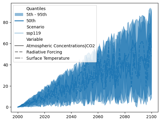
Calculate quantiles within plotting function
We can use plumeplot directly to plot quantiles. This will calculate the quantiles as part of
making the plot so if you’re doing this lots it might be faster to pre-calculate the quantiles,
then make the plot instead (see below)
Note that in this case the default setttings in plumeplot don’t produce anything that helpful,
we show how to modify them in the cell below.
runs.plumeplot(quantile_over="run_id")
/home/docs/checkouts/readthedocs.org/user_builds/scmdata/checkouts/stable/src/scmdata/run.py:197: PerformanceWarning: DataFrame is highly fragmented.  This is usually the result of calling `frame.insert` many times, which has poor performance.  Consider joining all columns at once using pd.concat(axis=1) instead. To get a de-fragmented frame, use `newframe = frame.copy()`
  df.reset_index(inplace=True)
(<Axes: >,
 [<matplotlib.patches.Patch at 0x7fb0ef1aaca0>,
  <matplotlib.collections.PolyCollection at 0x7fb0ef1cf1c0>,
  <matplotlib.lines.Line2D at 0x7fb0eef52f70>,
  <matplotlib.patches.Patch at 0x7fb0ef1354c0>,
  <matplotlib.lines.Line2D at 0x7fb0ef15efd0>,
  <matplotlib.patches.Patch at 0x7fb0ef135b20>,
  <matplotlib.lines.Line2D at 0x7fb0ef1358e0>,
  <matplotlib.lines.Line2D at 0x7fb0ef1358b0>,
  <matplotlib.lines.Line2D at 0x7fb0ef13bdf0>])
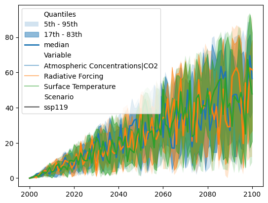
runs.plumeplot(
    quantile_over="run_id",
    quantiles_plumes=[
        ((0.05, 0.95), 0.2),
        ((0.17, 0.83), 0.5),
        (("median",), 1.0),
    ],
    hue_var="variable",
    hue_label="Variable",
    style_var="scenario",
    style_label="Scenario",
)
(<Axes: >,
 [<matplotlib.patches.Patch at 0x7fb0ec6b4580>,
  <matplotlib.collections.PolyCollection at 0x7fb0ec6c3730>,
  <matplotlib.collections.PolyCollection at 0x7fb0eae7b4f0>,
  <matplotlib.lines.Line2D at 0x7fb0eae08f70>,
  <matplotlib.patches.Patch at 0x7fb0eae84fd0>,
  <matplotlib.lines.Line2D at 0x7fb0eae4aeb0>,
  <matplotlib.lines.Line2D at 0x7fb0eae4af10>,
  <matplotlib.lines.Line2D at 0x7fb0eae69f70>,
  <matplotlib.patches.Patch at 0x7fb0eae848b0>,
  <matplotlib.lines.Line2D at 0x7fb0eae84f70>])
Pre-calculated quantiles
Alternately, we can cast the output of quantiles_over to an ScmRun object for ease of
filtering and plotting.
summary_stats_scmrun = ScmRun(summary_stats)
summary_stats_scmrun
<ScmRun (timeseries: 21, timepoints: 101)>
Time:
	Start: 2000-01-01T00:00:00
	End: 2100-01-01T00:00:00
Meta:
	      model quantile region scenario   unit                        variable
	0   example     0.05  World   ssp119    ppm  Atmospheric Concentrations|CO2
	1   example     0.05  World   ssp119  W/m^2               Radiative Forcing
	2   example     0.05  World   ssp119      K             Surface Temperature
	3   example     0.17  World   ssp119    ppm  Atmospheric Concentrations|CO2
	4   example     0.17  World   ssp119  W/m^2               Radiative Forcing
	5   example     0.17  World   ssp119      K             Surface Temperature
	6   example      0.5  World   ssp119    ppm  Atmospheric Concentrations|CO2
	7   example      0.5  World   ssp119  W/m^2               Radiative Forcing
	8   example      0.5  World   ssp119      K             Surface Temperature
	9   example     0.83  World   ssp119    ppm  Atmospheric Concentrations|CO2
	10  example     0.83  World   ssp119  W/m^2               Radiative Forcing
	11  example     0.83  World   ssp119      K             Surface Temperature
	12  example     0.95  World   ssp119    ppm  Atmospheric Concentrations|CO2
	13  example     0.95  World   ssp119  W/m^2               Radiative Forcing
	14  example     0.95  World   ssp119      K             Surface Temperature
	15  example     mean  World   ssp119    ppm  Atmospheric Concentrations|CO2
	16  example     mean  World   ssp119  W/m^2               Radiative Forcing
	17  example     mean  World   ssp119      K             Surface Temperature
	18  example   median  World   ssp119    ppm  Atmospheric Concentrations|CO2
	19  example   median  World   ssp119  W/m^2               Radiative Forcing
	20  example   median  World   ssp119      K             Surface Temperature
As discussed above, casting the output of quantiles_over to an ScmRun object helps avoid
repeatedly calculating the quantiles.
summary_stats_scmrun.plumeplot(
    quantiles_plumes=[
        ((0.05, 0.95), 0.2),
        ((0.17, 0.83), 0.5),
        (("median",), 1.0),
    ],
    hue_var="variable",
    hue_label="Variable",
    style_var="scenario",
    style_label="Scenario",
    pre_calculated=True,
)
(<Axes: >,
 [<matplotlib.patches.Patch at 0x7fb0eadf0df0>,
  <matplotlib.collections.PolyCollection at 0x7fb0ead4adf0>,
  <matplotlib.collections.PolyCollection at 0x7fb0eadc1be0>,
  <matplotlib.lines.Line2D at 0x7fb0eadc1a30>,
  <matplotlib.patches.Patch at 0x7fb0eadb66a0>,
  <matplotlib.lines.Line2D at 0x7fb0eadb6550>,
  <matplotlib.lines.Line2D at 0x7fb0eadb6e50>,
  <matplotlib.lines.Line2D at 0x7fb0eadb6fa0>,
  <matplotlib.patches.Patch at 0x7fb0eadb6760>,
  <matplotlib.lines.Line2D at 0x7fb0eadb6790>])
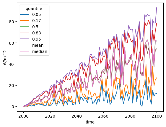
If we don’t want a plume plot, we can always our standard lineplot method.
summary_stats_scmrun.filter(variable="Radiative Forcing").lineplot(hue="quantile")
<Axes: xlabel='time', ylabel='W/m^2'>
groupby
The groupby method allows us to group the data by columns in scmrun.meta and then perform
operations. An example is given below.
variable_means = []
for vdf in runs.groupby("variable"):
    vdf_mean = vdf.timeseries().mean(axis=0)
    vdf_mean.name = vdf.get_unique_meta("variable", True)
    variable_means.append(vdf_mean)

pd.DataFrame(variable_means)
| time | 2000-01-01 | 2001-01-01 | 2002-01-01 | 2003-01-01 | 2004-01-01 | 2005-01-01 | 2006-01-01 | 2007-01-01 | 2008-01-01 | 2009-01-01 | ... | 2091-01-01 | 2092-01-01 | 2093-01-01 | 2094-01-01 | 2095-01-01 | 2096-01-01 | 2097-01-01 | 2098-01-01 | 2099-01-01 | 2100-01-01 |
|---|---|---|---|---|---|---|---|---|---|---|---|---|---|---|---|---|---|---|---|---|---|
| Atmospheric Concentrations|CO2 | 0.0 | 0.633726 | 0.820140 | 1.958988 | 2.226479 | 1.900248 | 2.518336 | 4.844826 | 3.766397 | 2.869477 | ... | 45.683007 | 42.843922 | 40.569624 | 46.601360 | 41.163366 | 44.988548 | 49.392486 | 53.709420 | 58.009569 | 54.531307 |
| Radiative Forcing | 0.0 | 0.454844 | 0.838021 | 0.802832 | 1.674571 | 2.628700 | 2.905800 | 4.296218 | 3.954549 | 5.279299 | ... | 52.578809 | 58.972332 | 49.857185 | 55.098508 | 46.207773 | 26.216435 | 52.611759 | 40.653964 | 53.058094 | 54.244386 |
| Surface Temperature | 0.0 | 0.358206 | 1.041445 | 1.764363 | 1.417427 | 2.316142 | 3.369883 | 2.818531 | 3.782787 | 5.052724 | ... | 38.278119 | 38.382656 | 44.063500 | 44.698675 | 42.390491 | 35.858052 | 31.400987 | 61.640357 | 53.662404 | 48.521514 |
3 rows × 101 columns
groupby_all_except
The groupby_all_except method allows us to group the data by all columns in scmrun.meta
except for a certain set. Like with groupby, we can then use the groups to perform operations.
An example is given below. Note that, in most cases, using process_over is likely to be more
useful.
ensemble_means = []
for edf in runs.groupby_all_except("run_id"):
    edf_mean = edf.timeseries().mean(axis=0)
    edf_mean.name = edf.get_unique_meta("variable", True)
    ensemble_means.append(edf_mean)

pd.DataFrame(ensemble_means)
| time | 2000-01-01 | 2001-01-01 | 2002-01-01 | 2003-01-01 | 2004-01-01 | 2005-01-01 | 2006-01-01 | 2007-01-01 | 2008-01-01 | 2009-01-01 | ... | 2091-01-01 | 2092-01-01 | 2093-01-01 | 2094-01-01 | 2095-01-01 | 2096-01-01 | 2097-01-01 | 2098-01-01 | 2099-01-01 | 2100-01-01 |
|---|---|---|---|---|---|---|---|---|---|---|---|---|---|---|---|---|---|---|---|---|---|
| Surface Temperature | 0.0 | 0.358206 | 1.041445 | 1.764363 | 1.417427 | 2.316142 | 3.369883 | 2.818531 | 3.782787 | 5.052724 | ... | 38.278119 | 38.382656 | 44.063500 | 44.698675 | 42.390491 | 35.858052 | 31.400987 | 61.640357 | 53.662404 | 48.521514 |
| Radiative Forcing | 0.0 | 0.454844 | 0.838021 | 0.802832 | 1.674571 | 2.628700 | 2.905800 | 4.296218 | 3.954549 | 5.279299 | ... | 52.578809 | 58.972332 | 49.857185 | 55.098508 | 46.207773 | 26.216435 | 52.611759 | 40.653964 | 53.058094 | 54.244386 |
| Atmospheric Concentrations|CO2 | 0.0 | 0.633726 | 0.820140 | 1.958988 | 2.226479 | 1.900248 | 2.518336 | 4.844826 | 3.766397 | 2.869477 | ... | 45.683007 | 42.843922 | 40.569624 | 46.601360 | 41.163366 | 44.988548 | 49.392486 | 53.709420 | 58.009569 | 54.531307 |
3 rows × 101 columns
As we said, in most cases using process_over is likely to be more useful. For example the above
can be done using process_over in one line (and more metadata is retained).
runs.process_over("run_id", "mean")
| time | 2000-01-01 | 2001-01-01 | 2002-01-01 | 2003-01-01 | 2004-01-01 | 2005-01-01 | 2006-01-01 | 2007-01-01 | 2008-01-01 | 2009-01-01 | ... | 2091-01-01 | 2092-01-01 | 2093-01-01 | 2094-01-01 | 2095-01-01 | 2096-01-01 | 2097-01-01 | 2098-01-01 | 2099-01-01 | 2100-01-01 | ||||
|---|---|---|---|---|---|---|---|---|---|---|---|---|---|---|---|---|---|---|---|---|---|---|---|---|---|
| model | region | scenario | unit | variable | |||||||||||||||||||||
| example | World | ssp119 | ppm | Atmospheric Concentrations|CO2 | 0.0 | 0.633726 | 0.820140 | 1.958988 | 2.226479 | 1.900248 | 2.518336 | 4.844826 | 3.766397 | 2.869477 | ... | 45.683007 | 42.843922 | 40.569624 | 46.601360 | 41.163366 | 44.988548 | 49.392486 | 53.709420 | 58.009569 | 54.531307 |
| W/m^2 | Radiative Forcing | 0.0 | 0.454844 | 0.838021 | 0.802832 | 1.674571 | 2.628700 | 2.905800 | 4.296218 | 3.954549 | 5.279299 | ... | 52.578809 | 58.972332 | 49.857185 | 55.098508 | 46.207773 | 26.216435 | 52.611759 | 40.653964 | 53.058094 | 54.244386 | |||
| K | Surface Temperature | 0.0 | 0.358206 | 1.041445 | 1.764363 | 1.417427 | 2.316142 | 3.369883 | 2.818531 | 3.782787 | 5.052724 | ... | 38.278119 | 38.382656 | 44.063500 | 44.698675 | 42.390491 | 35.858052 | 31.400987 | 61.640357 | 53.662404 | 48.521514 |
3 rows × 101 columns