import traceback
import warnings

import matplotlib.pyplot as plt
import pandas as pd

from scmdata import ScmRun, run_append

/tmp/ipykernel_782/1318481154.py:5: DeprecationWarning: 
Pyarrow will become a required dependency of pandas in the next major release of pandas (pandas 3.0),
(to allow more performant data types, such as the Arrow string type, and better interoperability with other libraries)
but was not found to be installed on your system.
If this would cause problems for you,
please provide us feedback at https://github.com/pandas-dev/pandas/issues/54466
        
  import pandas as pd
/home/docs/checkouts/readthedocs.org/user_builds/scmdata/checkouts/stable/src/scmdata/database/_database.py:9: TqdmWarning: IProgress not found. Please update jupyter and ipywidgets. See https://ipywidgets.readthedocs.io/en/stable/user_install.html
  import tqdm.autonotebook as tqdman

Operations

scmdata has limited support for operations with ScmRun instances. Here we provide examples of how to use them.

Available operations

At present, the following options are available:

• add

• subtract

• divide

• multiply

• integrate (sum and trapizoidal)

• change per unit time (numerical differentiation essentially)

• calculate linear regression

• shift median of an ensemble

These operations are unit aware so are fairly powerful.

Load some data

We first load some test data.

db_emms = ScmRun("rcp26_emissions.csv", lowercase_cols=True)
db_emms.tail()

				time	1765-01-01 00:00:00	1766-01-01 00:00:00	1767-01-01 00:00:00	1768-01-01 00:00:00	1769-01-01 00:00:00	1770-01-01 00:00:00	1771-01-01 00:00:00	1772-01-01 00:00:00	1773-01-01 00:00:00	1774-01-01 00:00:00	...	2491-01-01 00:00:00	2492-01-01 00:00:00	2493-01-01 00:00:00	2494-01-01 00:00:00	2495-01-01 00:00:00	2496-01-01 00:00:00	2497-01-01 00:00:00	2498-01-01 00:00:00	2499-01-01 00:00:00	2500-01-01 00:00:00
model	region	scenario	unit	variable
IMAGE	World	RCP26	Mt NMVOC / yr	Emissions|NMVOC	0.0	1.596875	2.292316	2.988648	3.685897	4.384091	5.083260	5.783435	6.484645	7.186924	...	125.5104	125.5104	125.5104	125.5104	125.5104	125.5104	125.5104	125.5104	125.5104	125.5104
			Mt N / yr	Emissions|NOx	0.0	0.109502	0.168038	0.226625	0.285264	0.343956	0.402704	0.461508	0.520371	0.579294	...	15.9895	15.9895	15.9895	15.9895	15.9895	15.9895	15.9895	15.9895	15.9895	15.9895
			Mt OC / yr	Emissions|OC	0.0	0.565920	0.781468	0.997361	1.213611	1.430229	1.647226	1.864613	2.082403	2.300608	...	25.3311	25.3311	25.3311	25.3311	25.3311	25.3311	25.3311	25.3311	25.3311	25.3311
			kt SF6 / yr	Emissions|SF6	0.0	0.000000	0.000000	0.000000	0.000000	0.000000	0.000000	0.000000	0.000000	0.000000	...	0.0442	0.0442	0.0442	0.0442	0.0442	0.0442	0.0442	0.0442	0.0442	0.0442
			Mt S / yr	Emissions|SOx	0.0	0.098883	0.116306	0.133811	0.151398	0.169070	0.186831	0.204683	0.222628	0.240670	...	6.4552	6.4552	6.4552	6.4552	6.4552	6.4552	6.4552	6.4552	6.4552	6.4552

5 rows × 736 columns

db_forcing = ScmRun(
    "rcmip-radiative-forcing-annual-means-v4-0-0.csv", lowercase_cols=True
).drop_meta(["mip_era", "activity_id"], inplace=False)

db_forcing.head()

				time	1750-01-01 00:00:00	1751-01-01 00:00:00	1752-01-01 00:00:00	1753-01-01 00:00:00	1754-01-01 00:00:00	1755-01-01 00:00:00	1756-01-01 00:00:00	1757-01-01 00:00:00	1758-01-01 00:00:00	1759-01-01 00:00:00	...	2491-01-01 00:00:00	2492-01-01 00:00:00	2493-01-01 00:00:00	2494-01-01 00:00:00	2495-01-01 00:00:00	2496-01-01 00:00:00	2497-01-01 00:00:00	2498-01-01 00:00:00	2499-01-01 00:00:00	2500-01-01 00:00:00
model	region	scenario	unit	variable
AIM	World	rcp60	W/m^2	Radiative Forcing	NaN	NaN	NaN	NaN	NaN	NaN	NaN	NaN	NaN	NaN	...	5.993838	5.993838	5.993838	5.993838	5.993838	5.993838	5.993838	5.993838	5.993838	5.993838
				Radiative Forcing|Anthropogenic	NaN	NaN	NaN	NaN	NaN	NaN	NaN	NaN	NaN	NaN	...	5.890082	5.890082	5.890082	5.890082	5.890082	5.890082	5.890082	5.890082	5.890082	5.890082
				Radiative Forcing|Anthropogenic|Aerosols	NaN	NaN	NaN	NaN	NaN	NaN	NaN	NaN	NaN	NaN	...	-0.603691	-0.603691	-0.603691	-0.603691	-0.603691	-0.603691	-0.603691	-0.603691	-0.603691	-0.603691
				Radiative Forcing|Anthropogenic|Aerosols|Aerosols-cloud Interactions	NaN	NaN	NaN	NaN	NaN	NaN	NaN	NaN	NaN	NaN	...	-0.465404	-0.465404	-0.465404	-0.465404	-0.465404	-0.465404	-0.465404	-0.465404	-0.465404	-0.465404
				Radiative Forcing|Anthropogenic|Aerosols|Aerosols-radiation Interactions	NaN	NaN	NaN	NaN	NaN	NaN	NaN	NaN	NaN	NaN	...	-0.138286	-0.138286	-0.138286	-0.138286	-0.138286	-0.138286	-0.138286	-0.138286	-0.138286	-0.138286

5 rows × 751 columns

Add

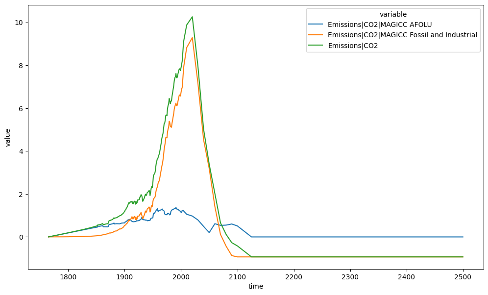
A very simple example is adding two variables together. For example, below we calculate total CO\(_2\) emissions for the RCP2.6 scenario.

emms_co2 = db_emms.filter(variable="Emissions|CO2|MAGICC Fossil and Industrial").add(
    db_emms.filter(variable="Emissions|CO2|MAGICC AFOLU"),
    op_cols={"variable": "Emissions|CO2"},
)
emms_co2.head()

				time	1765-01-01 00:00:00	1766-01-01 00:00:00	1767-01-01 00:00:00	1768-01-01 00:00:00	1769-01-01 00:00:00	1770-01-01 00:00:00	1771-01-01 00:00:00	1772-01-01 00:00:00	1773-01-01 00:00:00	1774-01-01 00:00:00	...	2491-01-01 00:00:00	2492-01-01 00:00:00	2493-01-01 00:00:00	2494-01-01 00:00:00	2495-01-01 00:00:00	2496-01-01 00:00:00	2497-01-01 00:00:00	2498-01-01 00:00:00	2499-01-01 00:00:00	2500-01-01 00:00:00
model	region	scenario	unit	variable
IMAGE	World	RCP26	C * gigametric_ton / a	Emissions|CO2	0.003	0.008338	0.013677	0.019015	0.024353	0.029691	0.03603	0.041368	0.046706	0.052045	...	-0.9308	-0.9308	-0.9308	-0.9308	-0.9308	-0.9308	-0.9308	-0.9308	-0.9308	-0.9308

1 rows × 736 columns

ax = plt.figure(figsize=(12, 7)).add_subplot(111)
plt_df = run_append([db_emms, emms_co2])
plt_df.filter(variable="*CO2*").lineplot(hue="variable", ax=ax)

<Axes: xlabel='time', ylabel='value'>

The op_cols argument tells scmdata which columns to ignore when aligning the data and what value to give this column in the output. So we could do the same calculation but give the output a different name as shown below.

emms_co2_different_name = db_emms.filter(
    variable="Emissions|CO2|MAGICC Fossil and Industrial"
).add(
    db_emms.filter(variable="Emissions|CO2|MAGICC AFOLU"),
    op_cols={"variable": "Emissions|CO2|Total"},
)
emms_co2_different_name.head()

				time	1765-01-01 00:00:00	1766-01-01 00:00:00	1767-01-01 00:00:00	1768-01-01 00:00:00	1769-01-01 00:00:00	1770-01-01 00:00:00	1771-01-01 00:00:00	1772-01-01 00:00:00	1773-01-01 00:00:00	1774-01-01 00:00:00	...	2491-01-01 00:00:00	2492-01-01 00:00:00	2493-01-01 00:00:00	2494-01-01 00:00:00	2495-01-01 00:00:00	2496-01-01 00:00:00	2497-01-01 00:00:00	2498-01-01 00:00:00	2499-01-01 00:00:00	2500-01-01 00:00:00
model	region	scenario	unit	variable
IMAGE	World	RCP26	C * gigametric_ton / a	Emissions|CO2|Total	0.003	0.008338	0.013677	0.019015	0.024353	0.029691	0.03603	0.041368	0.046706	0.052045	...	-0.9308	-0.9308	-0.9308	-0.9308	-0.9308	-0.9308	-0.9308	-0.9308	-0.9308	-0.9308

1 rows × 736 columns

Subtract

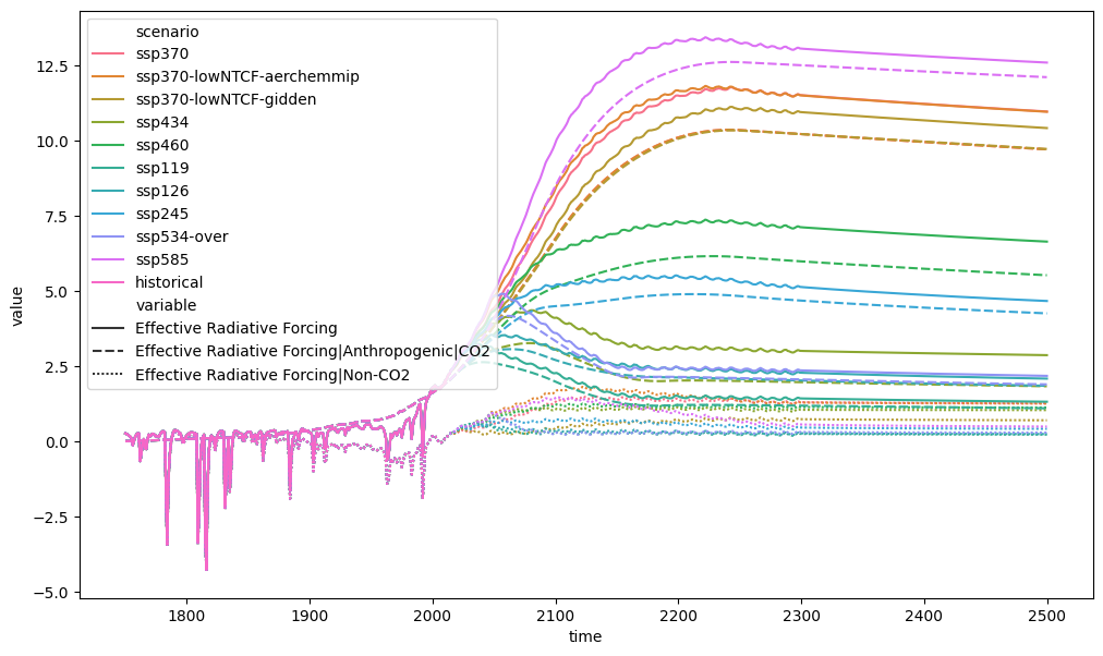
Subtraction works much the same way. Below we calculate the total effective radiative forcing and CO\(_2\) effective radiative forcing in the RCMIP data.

non_co2_rf = db_forcing.filter(variable="Effective Radiative Forcing").subtract(
    db_forcing.filter(variable="Effective Radiative Forcing|Anthropogenic|CO2"),
    op_cols={"variable": "Effective Radiative Forcing|Non-CO2"},
)
non_co2_rf.head()

				time	1750-01-01 00:00:00	1751-01-01 00:00:00	1752-01-01 00:00:00	1753-01-01 00:00:00	1754-01-01 00:00:00	1755-01-01 00:00:00	1756-01-01 00:00:00	1757-01-01 00:00:00	1758-01-01 00:00:00	1759-01-01 00:00:00	...	2491-01-01 00:00:00	2492-01-01 00:00:00	2493-01-01 00:00:00	2494-01-01 00:00:00	2495-01-01 00:00:00	2496-01-01 00:00:00	2497-01-01 00:00:00	2498-01-01 00:00:00	2499-01-01 00:00:00	2500-01-01 00:00:00
model	region	scenario	unit	variable
AIM/CGE	World	ssp370	watt / meter ** 2	Effective Radiative Forcing|Non-CO2	0.259367	0.241965	0.213009	0.177158	0.142201	0.094554	-0.137892	0.010089	0.140326	0.218701	...	1.259420	1.259326	1.259229	1.259130	1.259034	1.258938	1.258848	1.258752	1.258657	1.258609
		ssp370-lowNTCF-aerchemmip	watt / meter ** 2	Effective Radiative Forcing|Non-CO2	0.259367	0.241965	0.213009	0.177158	0.142201	0.094554	-0.137892	0.010089	0.140326	0.218701	...	1.250176	1.250081	1.249985	1.249885	1.249789	1.249693	1.249603	1.249508	1.249412	1.249365
		ssp370-lowNTCF-gidden	watt / meter ** 2	Effective Radiative Forcing|Non-CO2	0.259367	0.241965	0.213009	0.177158	0.142201	0.094554	-0.137892	0.010089	0.140326	0.218701	...	0.695533	0.695413	0.695297	0.695182	0.695067	0.694952	0.694830	0.694715	0.694600	0.694547
GCAM4	World	ssp434	watt / meter ** 2	Effective Radiative Forcing|Non-CO2	0.259367	0.241965	0.213009	0.177158	0.142201	0.094554	-0.137892	0.010089	0.140326	0.218701	...	1.033839	1.033813	1.033785	1.033760	1.033735	1.033710	1.033683	1.033658	1.033626	1.033616
		ssp460	watt / meter ** 2	Effective Radiative Forcing|Non-CO2	0.259367	0.241965	0.213009	0.177158	0.142201	0.094554	-0.137892	0.010089	0.140326	0.218701	...	1.116804	1.116756	1.116709	1.116659	1.116612	1.116565	1.116519	1.116472	1.116429	1.116403

5 rows × 751 columns

ax = plt.figure(figsize=(12, 7)).add_subplot(111)
plt_df_forcing = run_append([db_forcing, non_co2_rf])
plt_df_forcing.filter(
    variable=["Effective Radiative Forcing", "Effective*CO2*"]
).lineplot(style="variable")

<Axes: xlabel='time', ylabel='value'>

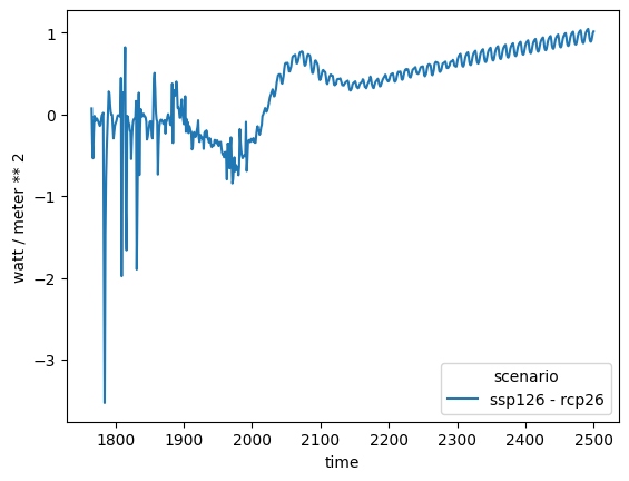
We could also calculate the difference between some SSP and RCP scenarios. The first thing to try would be to simply subtract the SSP126 total effective radiative forcing from the RCP26 total radiative forcing.

try:
    ssp126_minus_rcp26 = db_forcing.filter(
        scenario="ssp126", variable="Effective Radiative Forcing"
    ).subtract(
        db_forcing.filter(scenario="rcp26", variable="Radiative Forcing"),
        op_cols={
            "scenario": "ssp126 - rcp26",
        },
    )
except KeyError:
    traceback.print_exc(limit=0, chain=False)

KeyError: "No equivalent in `other` for [('model', 'IMAGE'), ('region', 'World'), ('variable', 'Effective Radiative Forcing')]"

Doing this gives us a KeyError. The reason is that the SSP126 variable is Effective Radiative Forcing whilst the RCP26 variable is Radiative Forcing hence the two datasets don’t align. We can work around this using the op_cols argument.

ssp126_minus_rcp26 = db_forcing.filter(
    scenario="ssp126", variable="Effective Radiative Forcing"
).subtract(
    db_forcing.filter(scenario="rcp26", variable="Radiative Forcing"),
    op_cols={
        "scenario": "ssp126 - rcp26",
        "variable": "RF",
    },
)
ssp126_minus_rcp26.lineplot()

<Axes: xlabel='time', ylabel='watt / meter ** 2'>

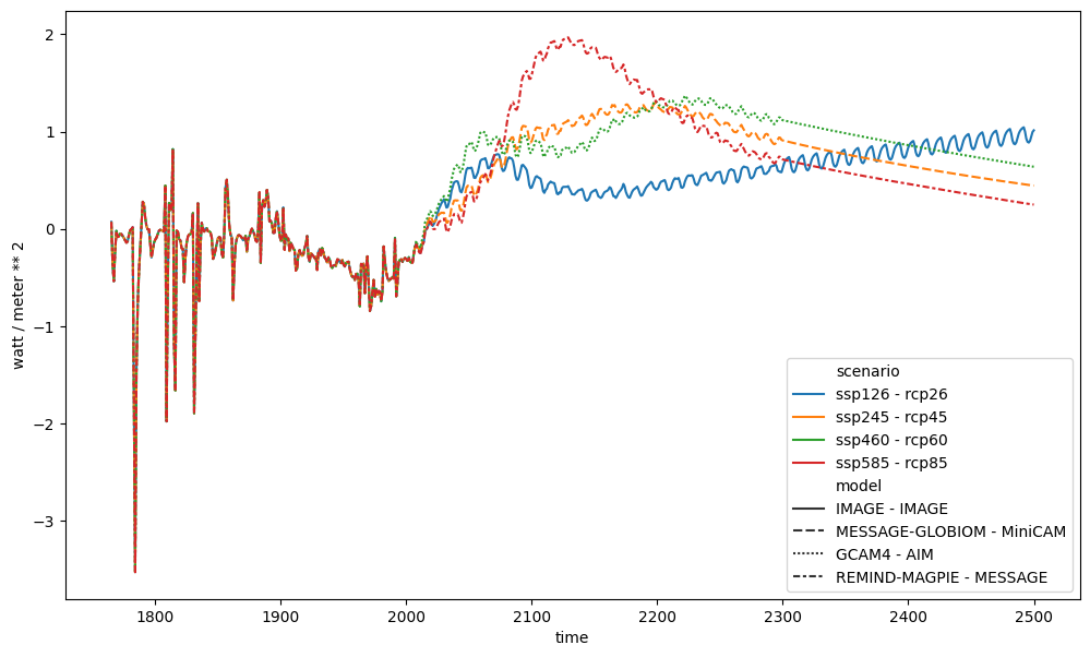
We could create plots of all the differences as shown below.

ssp_rcp_diffs = []
for target in ["26", "45", "60", "85"]:
    ssp = db_forcing.filter(
        scenario=f"ssp*{target}",
        variable="Effective Radiative Forcing",
    )
    ssp_scen = ssp.get_unique_meta("scenario", no_duplicates=True)
    ssp_model = ssp.get_unique_meta("model", no_duplicates=True)

    rcp = db_forcing.filter(scenario=f"rcp{target}", variable="Radiative Forcing")
    rcp_scen = rcp.get_unique_meta("scenario", no_duplicates=True)
    rcp_model = rcp.get_unique_meta("model", no_duplicates=True)

    ssp_rcp_diff = ssp.subtract(
        rcp,
        op_cols={
            "scenario": f"{ssp_scen} - {rcp_scen}",
            "model": f"{ssp_model} - {rcp_model}",
            "variable": "RF",
        },
    )
    ssp_rcp_diffs.append(ssp_rcp_diff)

ssp_rcp_diffs = run_append(ssp_rcp_diffs)
ssp_rcp_diffs.head()

				time	1750-01-01 00:00:00	1751-01-01 00:00:00	1752-01-01 00:00:00	1753-01-01 00:00:00	1754-01-01 00:00:00	1755-01-01 00:00:00	1756-01-01 00:00:00	1757-01-01 00:00:00	1758-01-01 00:00:00	1759-01-01 00:00:00	...	2491-01-01 00:00:00	2492-01-01 00:00:00	2493-01-01 00:00:00	2494-01-01 00:00:00	2495-01-01 00:00:00	2496-01-01 00:00:00	2497-01-01 00:00:00	2498-01-01 00:00:00	2499-01-01 00:00:00	2500-01-01 00:00:00
model	region	scenario	unit	variable
IMAGE - IMAGE	World	ssp126 - rcp26	watt / meter ** 2	RF	NaN	NaN	NaN	NaN	NaN	NaN	NaN	NaN	NaN	NaN	...	1.036063	1.044192	0.998926	0.927014	0.894074	0.886604	0.904720	0.950169	0.995562	1.012583
MESSAGE-GLOBIOM - MiniCAM	World	ssp245 - rcp45	watt / meter ** 2	RF	NaN	NaN	NaN	NaN	NaN	NaN	NaN	NaN	NaN	NaN	...	0.460000	0.458162	0.456325	0.454487	0.452659	0.450835	0.449006	0.447191	0.445375	0.444465
GCAM4 - AIM	World	ssp460 - rcp60	watt / meter ** 2	RF	NaN	NaN	NaN	NaN	NaN	NaN	NaN	NaN	NaN	NaN	...	0.656893	0.654786	0.652687	0.650594	0.648503	0.646411	0.644319	0.642235	0.640155	0.639114
REMIND-MAGPIE - MESSAGE	World	ssp585 - rcp85	watt / meter ** 2	RF	NaN	NaN	NaN	NaN	NaN	NaN	NaN	NaN	NaN	NaN	...	0.266282	0.264204	0.262160	0.260144	0.258118	0.256072	0.254027	0.252006	0.250012	0.248969

4 rows × 751 columns

ax = plt.figure(figsize=(12, 7)).add_subplot(111)
ssp_rcp_diffs.lineplot(ax=ax, style="model")

<Axes: xlabel='time', ylabel='watt / meter ** 2'>

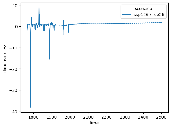
Divide

The divide (and multiply) operations clearly have to also be aware of units. Thanks to Pint’s pandas interface, this can happen automatically. For example, in our calculation below the units are automatically returned as dimensionless.

ssp126_to_rcp26 = db_forcing.filter(
    scenario="ssp126", variable="Effective Radiative Forcing"
).divide(
    db_forcing.filter(scenario="rcp26", variable="Radiative Forcing"),
    op_cols={
        "scenario": "ssp126 / rcp26",
        "variable": "RF",
    },
)
ssp126_to_rcp26.head()

				time	1750-01-01 00:00:00	1751-01-01 00:00:00	1752-01-01 00:00:00	1753-01-01 00:00:00	1754-01-01 00:00:00	1755-01-01 00:00:00	1756-01-01 00:00:00	1757-01-01 00:00:00	1758-01-01 00:00:00	1759-01-01 00:00:00	...	2491-01-01 00:00:00	2492-01-01 00:00:00	2493-01-01 00:00:00	2494-01-01 00:00:00	2495-01-01 00:00:00	2496-01-01 00:00:00	2497-01-01 00:00:00	2498-01-01 00:00:00	2499-01-01 00:00:00	2500-01-01 00:00:00
model	region	scenario	unit	variable
IMAGE	World	ssp126 / rcp26	dimensionless	RF	NaN	NaN	NaN	NaN	NaN	NaN	NaN	NaN	NaN	NaN	...	1.987642	2.003883	1.920958	1.802047	1.752583	1.742102	1.769413	1.841106	1.918814	1.949772

1 rows × 751 columns

ssp126_to_rcp26.lineplot()

<Axes: xlabel='time', ylabel='dimensionless'>

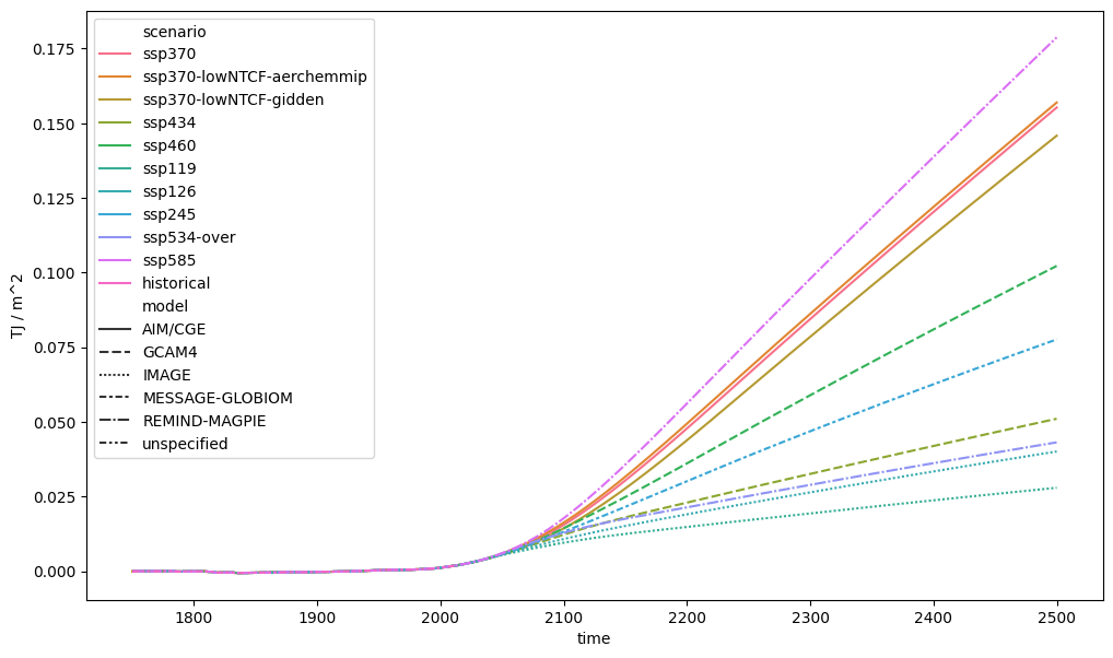
Integrate

We can also integrate our data. As previously, thanks to Pint and some other work, this operation is also unit aware.

There are two methods of integration available, cumtrapz and cumsum. The method that should be used depends on the data you are integrating, specifically whether the data are piecewise linear or piecewise constant.

Annual timeseries of emissions are piecewise constant (each value represents a total which is constant over an year) so should use the cumsum method.

Other output such as effective radiative forcing, concentrations or decadal timeseries of emissions, represent a point estimate or an average over a period. These timeseries are therefore piecewise linear and should use the cumtrapz method.

with warnings.catch_warnings():
    # Ignore warning about nans in the historical timeseries
    warnings.filterwarnings("ignore", module="scmdata.ops")

    # Radiative Forcings are piecewise-linear so `cumtrapz` should be used
    erf_integral = (
        db_forcing.filter(variable="Effective Radiative Forcing")
        .cumtrapz()
        .convert_unit("TJ / m^2")
    )

erf_integral

<ScmRun (timeseries: 11, timepoints: 751)>
Time:
	Start: 1750-01-01T00:00:00
	End: 2500-01-01T00:00:00
Meta:
	              model region                   scenario      unit  \
	0           AIM/CGE  World                     ssp370  TJ / m^2   
	1           AIM/CGE  World  ssp370-lowNTCF-aerchemmip  TJ / m^2   
	2           AIM/CGE  World      ssp370-lowNTCF-gidden  TJ / m^2   
	3             GCAM4  World                     ssp434  TJ / m^2   
	4             GCAM4  World                     ssp460  TJ / m^2   
	5             IMAGE  World                     ssp119  TJ / m^2   
	6             IMAGE  World                     ssp126  TJ / m^2   
	7   MESSAGE-GLOBIOM  World                     ssp245  TJ / m^2   
	8     REMIND-MAGPIE  World                ssp534-over  TJ / m^2   
	9     REMIND-MAGPIE  World                     ssp585  TJ / m^2   
	10      unspecified  World                 historical  TJ / m^2   
	
	                                  variable  
	0   Cumulative Effective Radiative Forcing  
	1   Cumulative Effective Radiative Forcing  
	2   Cumulative Effective Radiative Forcing  
	3   Cumulative Effective Radiative Forcing  
	4   Cumulative Effective Radiative Forcing  
	5   Cumulative Effective Radiative Forcing  
	6   Cumulative Effective Radiative Forcing  
	7   Cumulative Effective Radiative Forcing  
	8   Cumulative Effective Radiative Forcing  
	9   Cumulative Effective Radiative Forcing  
	10  Cumulative Effective Radiative Forcing  

ax = plt.figure(figsize=(12, 7)).add_subplot(111)
erf_integral.lineplot(ax=ax, style="model")

<Axes: xlabel='time', ylabel='TJ / m^2'>

with warnings.catch_warnings():
    # Ignore warning about nans in the historical timeseries
    warnings.filterwarnings("ignore", module="scmdata.ops")

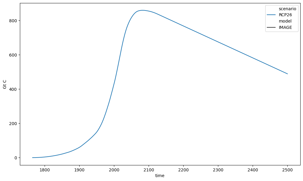
    # Emissions are piecewise-constant so `cumsum` should be used
    cumulative_emissions = emms_co2.cumsum().convert_unit("Gt C")

cumulative_emissions

<ScmRun (timeseries: 1, timepoints: 736)>
Time:
	Start: 1765-01-01T00:00:00
	End: 2500-01-01T00:00:00
Meta:
	   model region scenario  unit                  variable
	0  IMAGE  World    RCP26  Gt C  Cumulative Emissions|CO2

ax = plt.figure(figsize=(12, 7)).add_subplot(111)
cumulative_emissions.lineplot(ax=ax, style="model")

<Axes: xlabel='time', ylabel='Gt C'>

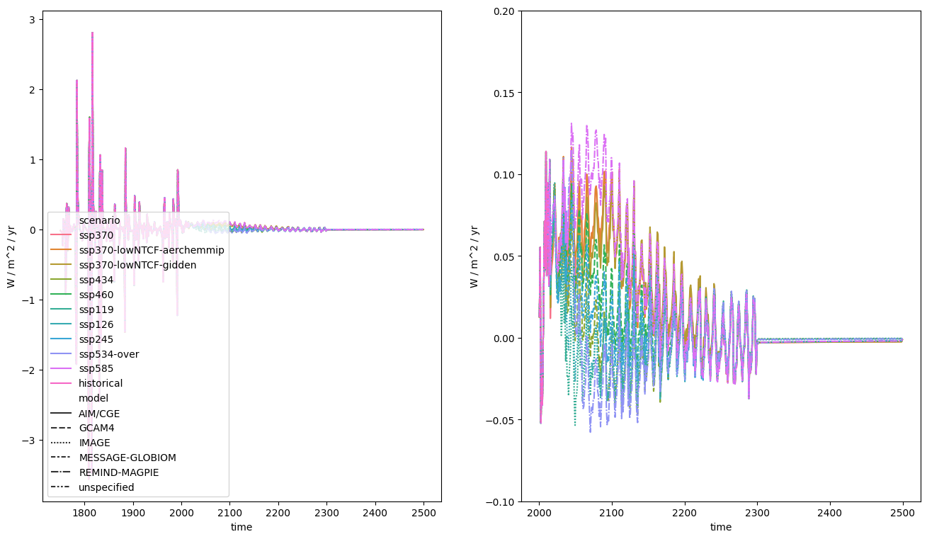
Time deltas

We can also calculate the change per unit time of our data. As previously, thanks to Pint and some other work, this operation is also unit aware.

with warnings.catch_warnings():
    # Ignore warning about nans in the historical timeseries
    warnings.filterwarnings("ignore", module="scmdata.ops")

    erf_delta = (
        db_forcing.filter(variable="Effective Radiative Forcing")
        .delta_per_delta_time()
        .convert_unit("W / m^2 / yr")
    )

erf_delta

<ScmRun (timeseries: 11, timepoints: 750)>
Time:
	Start: 1750-07-02T12:00:00
	End: 2499-07-02T12:00:00
Meta:
	              model region                   scenario          unit  \
	0           AIM/CGE  World                     ssp370  W / m^2 / yr   
	1           AIM/CGE  World  ssp370-lowNTCF-aerchemmip  W / m^2 / yr   
	2           AIM/CGE  World      ssp370-lowNTCF-gidden  W / m^2 / yr   
	3             GCAM4  World                     ssp434  W / m^2 / yr   
	4             GCAM4  World                     ssp460  W / m^2 / yr   
	5             IMAGE  World                     ssp119  W / m^2 / yr   
	6             IMAGE  World                     ssp126  W / m^2 / yr   
	7   MESSAGE-GLOBIOM  World                     ssp245  W / m^2 / yr   
	8     REMIND-MAGPIE  World                ssp534-over  W / m^2 / yr   
	9     REMIND-MAGPIE  World                     ssp585  W / m^2 / yr   
	10      unspecified  World                 historical  W / m^2 / yr   
	
	                             variable  
	0   Delta Effective Radiative Forcing  
	1   Delta Effective Radiative Forcing  
	2   Delta Effective Radiative Forcing  
	3   Delta Effective Radiative Forcing  
	4   Delta Effective Radiative Forcing  
	5   Delta Effective Radiative Forcing  
	6   Delta Effective Radiative Forcing  
	7   Delta Effective Radiative Forcing  
	8   Delta Effective Radiative Forcing  
	9   Delta Effective Radiative Forcing  
	10  Delta Effective Radiative Forcing  

fig, axes = plt.subplots(figsize=(16, 9), ncols=2)
erf_delta.lineplot(ax=axes[0], style="model")
erf_delta.filter(year=range(2000, 2500)).lineplot(
    ax=axes[1], style="model", legend=False
)
axes[1].set_ylim([-0.1, 0.2])

(-0.1, 0.2)

Regression

We can also calculate linear regressions of our data. As previously, thanks to Pint and some other work, this operation is also unit aware.

erf_total = db_forcing.filter(variable="Effective Radiative Forcing").filter(
    scenario="historical", keep=False
)
erf_total_for_reg = erf_total.filter(year=range(2010, 2050))

The default return type of linear_regression is a list of dictionaries.

linear_regression_raw = erf_total_for_reg.linear_regression()
type(linear_regression_raw)

list

type(linear_regression_raw[0])

dict

If we want, we can make a DataFrame from this list.

linear_regression_df = pd.DataFrame(linear_regression_raw)
linear_regression_df

	model	region	scenario	variable	gradient	intercept
0	AIM/CGE	World	ssp370	Effective Radiative Forcing	1.90373454366716e-09 watt / meter ** 2 / second	-0.42795992093158064 watt / meter ** 2
1	AIM/CGE	World	ssp370-lowNTCF-aerchemmip	Effective Radiative Forcing	2.196587535316519e-09 watt / meter ** 2 / second	-0.8448632244177651 watt / meter ** 2
2	AIM/CGE	World	ssp370-lowNTCF-gidden	Effective Radiative Forcing	1.599468808895454e-09 watt / meter ** 2 / second	0.057473556012937535 watt / meter ** 2
3	GCAM4	World	ssp434	Effective Radiative Forcing	1.513761825121089e-09 watt / meter ** 2 / second	0.21738181303589565 watt / meter ** 2
4	GCAM4	World	ssp460	Effective Radiative Forcing	1.8242980920680464e-09 watt / meter ** 2 / second	-0.2804321989242344 watt / meter ** 2
5	IMAGE	World	ssp119	Effective Radiative Forcing	8.935038882642927e-10 watt / meter ** 2 / second	1.2017704356912693 watt / meter ** 2
6	IMAGE	World	ssp126	Effective Radiative Forcing	1.2279126589716315e-09 watt / meter ** 2 / second	0.6544862441567445 watt / meter ** 2
7	MESSAGE-GLOBIOM	World	ssp245	Effective Radiative Forcing	1.6273999739537484e-09 watt / meter ** 2 / second	0.033991206478731474 watt / meter ** 2
8	REMIND-MAGPIE	World	ssp534-over	Effective Radiative Forcing	2.2703911252022266e-09 watt / meter ** 2 / second	-0.9204663925813401 watt / meter ** 2
9	REMIND-MAGPIE	World	ssp585	Effective Radiative Forcing	2.2626366011973838e-09 watt / meter ** 2 / second	-0.9168810372684146 watt / meter ** 2

Alternately, we can request only the gradients or only the intercepts (noting that intercepts are calculated using a time base which has zero at 1970-01-01 again).

erf_total_for_reg.linear_regression_gradient("W / m^2 / yr")

	model	region	scenario	variable	gradient	unit
0	AIM/CGE	World	ssp370	Effective Radiative Forcing	0.060077	W / m^2 / yr
1	AIM/CGE	World	ssp370-lowNTCF-aerchemmip	Effective Radiative Forcing	0.069319	W / m^2 / yr
2	AIM/CGE	World	ssp370-lowNTCF-gidden	Effective Radiative Forcing	0.050475	W / m^2 / yr
3	GCAM4	World	ssp434	Effective Radiative Forcing	0.047771	W / m^2 / yr
4	GCAM4	World	ssp460	Effective Radiative Forcing	0.057570	W / m^2 / yr
5	IMAGE	World	ssp119	Effective Radiative Forcing	0.028197	W / m^2 / yr
6	IMAGE	World	ssp126	Effective Radiative Forcing	0.038750	W / m^2 / yr
7	MESSAGE-GLOBIOM	World	ssp245	Effective Radiative Forcing	0.051357	W / m^2 / yr
8	REMIND-MAGPIE	World	ssp534-over	Effective Radiative Forcing	0.071648	W / m^2 / yr
9	REMIND-MAGPIE	World	ssp585	Effective Radiative Forcing	0.071403	W / m^2 / yr

erf_total_for_reg.linear_regression_intercept("W / m^2")

	model	region	scenario	variable	intercept	unit
0	AIM/CGE	World	ssp370	Effective Radiative Forcing	-0.427960	W / m^2
1	AIM/CGE	World	ssp370-lowNTCF-aerchemmip	Effective Radiative Forcing	-0.844863	W / m^2
2	AIM/CGE	World	ssp370-lowNTCF-gidden	Effective Radiative Forcing	0.057474	W / m^2
3	GCAM4	World	ssp434	Effective Radiative Forcing	0.217382	W / m^2
4	GCAM4	World	ssp460	Effective Radiative Forcing	-0.280432	W / m^2
5	IMAGE	World	ssp119	Effective Radiative Forcing	1.201770	W / m^2
6	IMAGE	World	ssp126	Effective Radiative Forcing	0.654486	W / m^2
7	MESSAGE-GLOBIOM	World	ssp245	Effective Radiative Forcing	0.033991	W / m^2
8	REMIND-MAGPIE	World	ssp534-over	Effective Radiative Forcing	-0.920466	W / m^2
9	REMIND-MAGPIE	World	ssp585	Effective Radiative Forcing	-0.916881	W / m^2

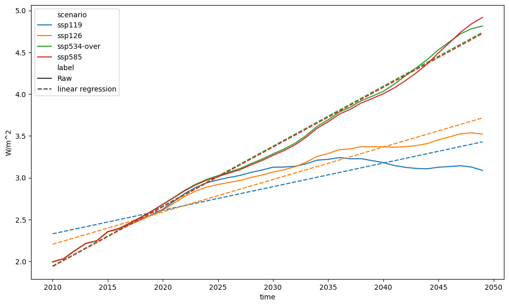
If we want to plot the regressions, we can request an ScmRun instance based on the linear regressions is returned using the linear_regression_scmrun method.

linear_regression = erf_total_for_reg.linear_regression_scmrun()
linear_regression["label"] = "linear regression"
linear_regression

<ScmRun (timeseries: 10, timepoints: 40)>
Time:
	Start: 2010-01-01T00:00:00
	End: 2049-01-01T00:00:00
Meta:
	               label            model region                   scenario  \
	0  linear regression          AIM/CGE  World                     ssp370   
	1  linear regression          AIM/CGE  World  ssp370-lowNTCF-aerchemmip   
	2  linear regression          AIM/CGE  World      ssp370-lowNTCF-gidden   
	3  linear regression            GCAM4  World                     ssp434   
	4  linear regression            GCAM4  World                     ssp460   
	5  linear regression            IMAGE  World                     ssp119   
	6  linear regression            IMAGE  World                     ssp126   
	7  linear regression  MESSAGE-GLOBIOM  World                     ssp245   
	8  linear regression    REMIND-MAGPIE  World                ssp534-over   
	9  linear regression    REMIND-MAGPIE  World                     ssp585   
	
	    unit                     variable  
	0  W/m^2  Effective Radiative Forcing  
	1  W/m^2  Effective Radiative Forcing  
	2  W/m^2  Effective Radiative Forcing  
	3  W/m^2  Effective Radiative Forcing  
	4  W/m^2  Effective Radiative Forcing  
	5  W/m^2  Effective Radiative Forcing  
	6  W/m^2  Effective Radiative Forcing  
	7  W/m^2  Effective Radiative Forcing  
	8  W/m^2  Effective Radiative Forcing  
	9  W/m^2  Effective Radiative Forcing  

erf_total_for_reg["label"] = "Raw"
pdf = run_append([erf_total_for_reg, linear_regression])

fig, axes = plt.subplots(figsize=(12, 7))
pdf.filter(scenario=["ssp1*", "ssp5*"]).lineplot(ax=axes, style="label")

<Axes: xlabel='time', ylabel='W/m^2'>

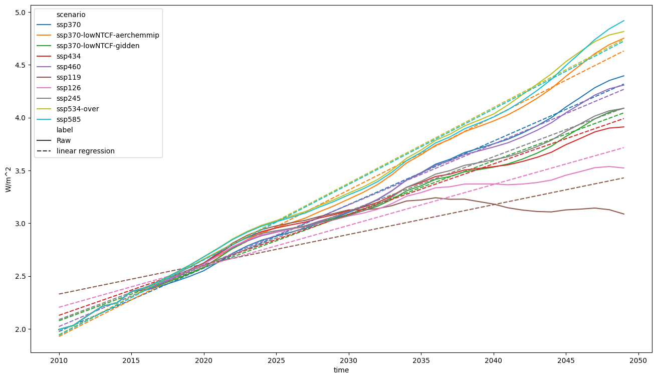
fig, axes = plt.subplots(figsize=(16, 9))
pdf.lineplot(ax=axes, style="label")

<Axes: xlabel='time', ylabel='W/m^2'>

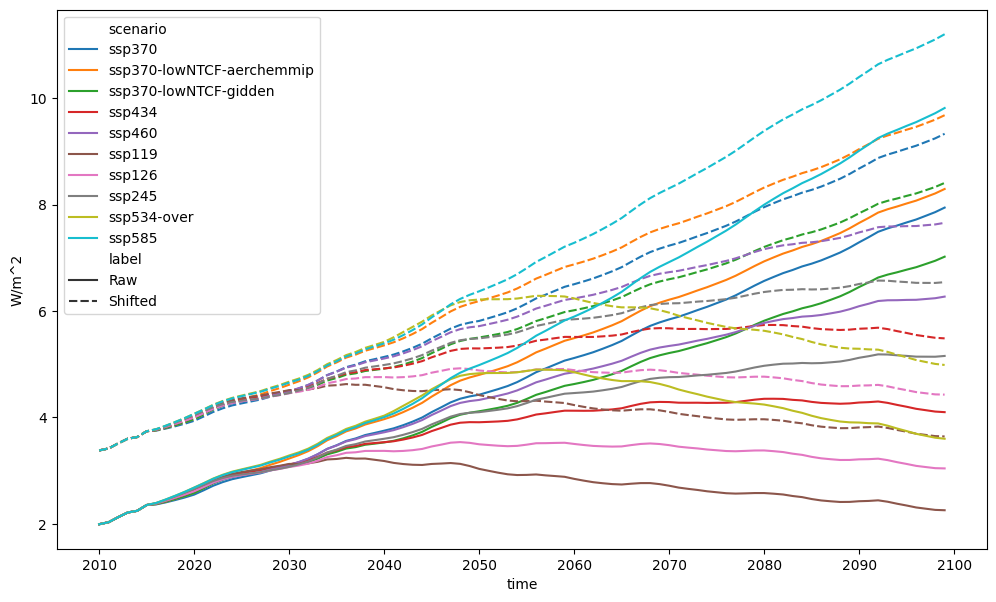
Shift median

Sometimes we wish to simply move an ensemble of timeseries so that its median matches some value, whilst preserving the spread of the ensemble. This can be done with the adjust_median_to_target method. For example, let’s say that we wanted to shift our ensemble of forcing values so that their 2030 median was equal to 4.5 (god knows why we would want to do this, but it will serve as an example).

erf_total = db_forcing.filter(variable="Effective Radiative Forcing").filter(
    scenario="historical", keep=False
)
erf_total_for_shift = erf_total.filter(year=range(2010, 2100))
erf_total_for_shift["label"] = "Raw"

erf_total_for_shift

<ScmRun (timeseries: 10, timepoints: 90)>
Time:
	Start: 2010-01-01T00:00:00
	End: 2099-01-01T00:00:00
Meta:
	    label            model region                   scenario   unit  \
	58    Raw          AIM/CGE  World                     ssp370  W/m^2   
	77    Raw          AIM/CGE  World  ssp370-lowNTCF-aerchemmip  W/m^2   
	96    Raw          AIM/CGE  World      ssp370-lowNTCF-gidden  W/m^2   
	115   Raw            GCAM4  World                     ssp434  W/m^2   
	134   Raw            GCAM4  World                     ssp460  W/m^2   
	211   Raw            IMAGE  World                     ssp119  W/m^2   
	230   Raw            IMAGE  World                     ssp126  W/m^2   
	307   Raw  MESSAGE-GLOBIOM  World                     ssp245  W/m^2   
	384   Raw    REMIND-MAGPIE  World                ssp534-over  W/m^2   
	403   Raw    REMIND-MAGPIE  World                     ssp585  W/m^2   
	
	                        variable  
	58   Effective Radiative Forcing  
	77   Effective Radiative Forcing  
	96   Effective Radiative Forcing  
	115  Effective Radiative Forcing  
	134  Effective Radiative Forcing  
	211  Effective Radiative Forcing  
	230  Effective Radiative Forcing  
	307  Effective Radiative Forcing  
	384  Effective Radiative Forcing  
	403  Effective Radiative Forcing  

erf_total_shifted = erf_total_for_shift.adjust_median_to_target(
    target=4.5,
    evaluation_period=2030,
    process_over=("scenario", "model"),
)
erf_total_shifted["label"] = "Shifted"

pdf = run_append([erf_total_for_shift, erf_total_shifted])

fig, axes = plt.subplots(figsize=(12, 7))
pdf.lineplot(ax=axes, style="label")

<Axes: xlabel='time', ylabel='W/m^2'>

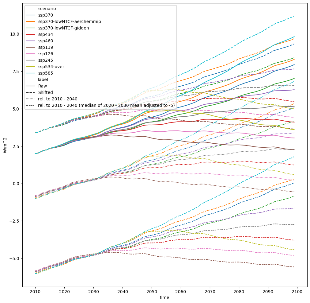
If we wanted, we could adjust the timeseries relative to some reference period first before doing the shift.

ref_period = range(2010, 2040 + 1)
erf_total_for_shift_rel_to_ref_period = erf_total_for_shift.relative_to_ref_period_mean(
    year=ref_period
)
erf_total_for_shift_rel_to_ref_period[
    "label"
] = f"rel. to {ref_period[0]} - {ref_period[-1]}"

target = -5
evaluation_period = range(2020, 2030 + 1)
erf_total_for_shift_rel_to_ref_period_shifted = (
    erf_total_for_shift_rel_to_ref_period.adjust_median_to_target(
        target=target,
        evaluation_period=evaluation_period,
        process_over=("scenario", "model"),
    )
)
erf_total_for_shift_rel_to_ref_period_shifted[
    "label"
] = "rel. to {} - {} (median of {} - {} mean adjusted to {})".format(
    ref_period[0],
    ref_period[-1],
    evaluation_period[0],
    evaluation_period[-1],
    target,
)

pdf = run_append(
    [
        erf_total_for_shift,
        erf_total_shifted,
        erf_total_for_shift_rel_to_ref_period,
        erf_total_for_shift_rel_to_ref_period_shifted,
    ]
)

fig, axes = plt.subplots(figsize=(12, 12))
pdf.lineplot(ax=axes, style="label")

<Axes: xlabel='time', ylabel='W/m^2'>