import pathlib
NetCDF handling
NetCDF formatted files are much faster to read and write for large datasets.
In order to make the most of this, the ScmRun objects have the ability to
read and write netCDF files.
import traceback
from tempfile import TemporaryDirectory

import numpy as np
import seaborn as sns
import xarray as xr

from scmdata.netcdf import nc_to_run
from scmdata.run import ScmRun, run_append
/home/docs/checkouts/readthedocs.org/user_builds/scmdata/checkouts/stable/src/scmdata/database/_database.py:9: TqdmWarning: IProgress not found. Please update jupyter and ipywidgets. See https://ipywidgets.readthedocs.io/en/stable/user_install.html
  import tqdm.autonotebook as tqdman
Helper bits and piecs
temp_directory = TemporaryDirectory()
generator = np.random.default_rng(0)
OUTPUT_DIR = pathlib.Path(temp_directory.name)

OUT_FNAME = OUTPUT_DIR / "out_runs.nc"
def new_timeseries(  # noqa: PLR0913
    n=100,
    count=1,
    model="example",
    scenario="ssp119",
    variable="Surface Temperature",
    unit="K",
    region="World",
    cls=ScmRun,
    **kwargs,
):
    """
    Create an example timeseries
    """
    data = generator.random((n, count)) * np.arange(n)[:, np.newaxis]
    index = 2000 + np.arange(n)
    return cls(
        data,
        columns={
            "model": model,
            "scenario": scenario,
            "variable": variable,
            "region": region,
            "unit": unit,
            **kwargs,
        },
        index=index,
    )
Let’s create an ScmRun which contains a few variables and a number of runs.
Such a dataframe would be used to store the results from an ensemble of
simple climate model runs.
runs = run_append(
    [
        new_timeseries(
            count=3,
            variable=[
                "Surface Temperature",
                "Atmospheric Concentrations|CO2",
                "Radiative Forcing",
            ],
            unit=["K", "ppm", "W/m^2"],
            run_id=run_id,
        )
        for run_id in range(10)
    ]
)
runs.metadata["source"] = "fake data"
runs
<ScmRun (timeseries: 30, timepoints: 100)>
Time:
	Start: 2000-01-01T00:00:00
	End: 2099-01-01T00:00:00
Meta:
	      model region  run_id scenario   unit                        variable
	0   example  World       0   ssp119      K             Surface Temperature
	1   example  World       0   ssp119    ppm  Atmospheric Concentrations|CO2
	2   example  World       0   ssp119  W/m^2               Radiative Forcing
	3   example  World       1   ssp119      K             Surface Temperature
	4   example  World       1   ssp119    ppm  Atmospheric Concentrations|CO2
	5   example  World       1   ssp119  W/m^2               Radiative Forcing
	6   example  World       2   ssp119      K             Surface Temperature
	7   example  World       2   ssp119    ppm  Atmospheric Concentrations|CO2
	8   example  World       2   ssp119  W/m^2               Radiative Forcing
	9   example  World       3   ssp119      K             Surface Temperature
	10  example  World       3   ssp119    ppm  Atmospheric Concentrations|CO2
	11  example  World       3   ssp119  W/m^2               Radiative Forcing
	12  example  World       4   ssp119      K             Surface Temperature
	13  example  World       4   ssp119    ppm  Atmospheric Concentrations|CO2
	14  example  World       4   ssp119  W/m^2               Radiative Forcing
	15  example  World       5   ssp119      K             Surface Temperature
	16  example  World       5   ssp119    ppm  Atmospheric Concentrations|CO2
	17  example  World       5   ssp119  W/m^2               Radiative Forcing
	18  example  World       6   ssp119      K             Surface Temperature
	19  example  World       6   ssp119    ppm  Atmospheric Concentrations|CO2
	20  example  World       6   ssp119  W/m^2               Radiative Forcing
	21  example  World       7   ssp119      K             Surface Temperature
	22  example  World       7   ssp119    ppm  Atmospheric Concentrations|CO2
	23  example  World       7   ssp119  W/m^2               Radiative Forcing
	24  example  World       8   ssp119      K             Surface Temperature
	25  example  World       8   ssp119    ppm  Atmospheric Concentrations|CO2
	26  example  World       8   ssp119  W/m^2               Radiative Forcing
	27  example  World       9   ssp119      K             Surface Temperature
	28  example  World       9   ssp119    ppm  Atmospheric Concentrations|CO2
	29  example  World       9   ssp119  W/m^2               Radiative Forcing
Reading/Writing to NetCDF4
Basics
Writing the runs to disk is easy. The one trick is that each variable and dimension combination must have unique metadata. If they do not, you will receive an error message like the below.
try:
    runs.to_nc(OUT_FNAME, dimensions=["region"])
except ValueError:
    traceback.print_exc(limit=0, chain=False)
ValueError: dimensions: `['region']` and extras: `[]` do not uniquely define the timeseries, please add extra dimensions and/or extras
In our dataset, there is more than one “run_id” per variable hence we need to use a different
dimension, run_id, because this will result in each variable’s remaining metadata being unique.
runs.to_nc(OUT_FNAME, dimensions=["run_id"])
/home/docs/checkouts/readthedocs.org/user_builds/scmdata/checkouts/stable/src/scmdata/_xarray.py:236: FutureWarning: The previous implementation of stack is deprecated and will be removed in a future version of pandas. See the What's New notes for pandas 2.1.0 for details. Specify future_stack=True to adopt the new implementation and silence this warning.
  else timeseries.T.stack(dimensions)
The output netCDF file can be read using the from_nc method, nc_to_run function or directly
using xarray.
runs_netcdf = ScmRun.from_nc(OUT_FNAME)
runs_netcdf
<ScmRun (timeseries: 30, timepoints: 100)>
Time:
	Start: 2000-01-01T00:00:00
	End: 2099-01-01T00:00:00
Meta:
	      model region  run_id scenario   unit                        variable
	0   example  World       0   ssp119      K             Surface Temperature
	1   example  World       0   ssp119    ppm  Atmospheric Concentrations|CO2
	2   example  World       0   ssp119  W/m^2               Radiative Forcing
	3   example  World       1   ssp119      K             Surface Temperature
	4   example  World       1   ssp119    ppm  Atmospheric Concentrations|CO2
	5   example  World       1   ssp119  W/m^2               Radiative Forcing
	6   example  World       2   ssp119      K             Surface Temperature
	7   example  World       2   ssp119    ppm  Atmospheric Concentrations|CO2
	8   example  World       2   ssp119  W/m^2               Radiative Forcing
	9   example  World       3   ssp119      K             Surface Temperature
	10  example  World       3   ssp119    ppm  Atmospheric Concentrations|CO2
	11  example  World       3   ssp119  W/m^2               Radiative Forcing
	12  example  World       4   ssp119      K             Surface Temperature
	13  example  World       4   ssp119    ppm  Atmospheric Concentrations|CO2
	14  example  World       4   ssp119  W/m^2               Radiative Forcing
	15  example  World       5   ssp119      K             Surface Temperature
	16  example  World       5   ssp119    ppm  Atmospheric Concentrations|CO2
	17  example  World       5   ssp119  W/m^2               Radiative Forcing
	18  example  World       6   ssp119      K             Surface Temperature
	19  example  World       6   ssp119    ppm  Atmospheric Concentrations|CO2
	20  example  World       6   ssp119  W/m^2               Radiative Forcing
	21  example  World       7   ssp119      K             Surface Temperature
	22  example  World       7   ssp119    ppm  Atmospheric Concentrations|CO2
	23  example  World       7   ssp119  W/m^2               Radiative Forcing
	24  example  World       8   ssp119      K             Surface Temperature
	25  example  World       8   ssp119    ppm  Atmospheric Concentrations|CO2
	26  example  World       8   ssp119  W/m^2               Radiative Forcing
	27  example  World       9   ssp119      K             Surface Temperature
	28  example  World       9   ssp119    ppm  Atmospheric Concentrations|CO2
	29  example  World       9   ssp119  W/m^2               Radiative Forcing
nc_to_run(ScmRun, OUT_FNAME)
<ScmRun (timeseries: 30, timepoints: 100)>
Time:
	Start: 2000-01-01T00:00:00
	End: 2099-01-01T00:00:00
Meta:
	      model region  run_id scenario   unit                        variable
	0   example  World       0   ssp119      K             Surface Temperature
	1   example  World       0   ssp119    ppm  Atmospheric Concentrations|CO2
	2   example  World       0   ssp119  W/m^2               Radiative Forcing
	3   example  World       1   ssp119      K             Surface Temperature
	4   example  World       1   ssp119    ppm  Atmospheric Concentrations|CO2
	5   example  World       1   ssp119  W/m^2               Radiative Forcing
	6   example  World       2   ssp119      K             Surface Temperature
	7   example  World       2   ssp119    ppm  Atmospheric Concentrations|CO2
	8   example  World       2   ssp119  W/m^2               Radiative Forcing
	9   example  World       3   ssp119      K             Surface Temperature
	10  example  World       3   ssp119    ppm  Atmospheric Concentrations|CO2
	11  example  World       3   ssp119  W/m^2               Radiative Forcing
	12  example  World       4   ssp119      K             Surface Temperature
	13  example  World       4   ssp119    ppm  Atmospheric Concentrations|CO2
	14  example  World       4   ssp119  W/m^2               Radiative Forcing
	15  example  World       5   ssp119      K             Surface Temperature
	16  example  World       5   ssp119    ppm  Atmospheric Concentrations|CO2
	17  example  World       5   ssp119  W/m^2               Radiative Forcing
	18  example  World       6   ssp119      K             Surface Temperature
	19  example  World       6   ssp119    ppm  Atmospheric Concentrations|CO2
	20  example  World       6   ssp119  W/m^2               Radiative Forcing
	21  example  World       7   ssp119      K             Surface Temperature
	22  example  World       7   ssp119    ppm  Atmospheric Concentrations|CO2
	23  example  World       7   ssp119  W/m^2               Radiative Forcing
	24  example  World       8   ssp119      K             Surface Temperature
	25  example  World       8   ssp119    ppm  Atmospheric Concentrations|CO2
	26  example  World       8   ssp119  W/m^2               Radiative Forcing
	27  example  World       9   ssp119      K             Surface Temperature
	28  example  World       9   ssp119    ppm  Atmospheric Concentrations|CO2
	29  example  World       9   ssp119  W/m^2               Radiative Forcing
xr.load_dataset(OUT_FNAME)
<xarray.Dataset>
Dimensions:                          (time: 100, run_id: 10)
Coordinates:
  * time                             (time) datetime64[ns] 2000-01-01 ... 209...
  * run_id                           (run_id) int64 0 1 2 3 4 5 6 7 8 9
Data variables:
    Surface_Temperature              (run_id, time) float64 0.0 ... 2.459
    Atmospheric_Concentrations__CO2  (run_id, time) float64 0.0 0.8133 ... 20.56
    Radiative_Forcing                (run_id, time) float64 0.0 0.9128 ... 29.75
Attributes:
    scmdata_metadata_scenario:  ssp119
    scmdata_metadata_model:     example
    scmdata_metadata_region:    World
    created_at:                 2024-01-29T07:18:01.855754
    _scmdata_version:           1.0.0
source: fake dataThe additional metadata in runs is also serialized and deserialized in the netCDF files. The
metadata of the loaded ScmRun will also contain some additional fields about the file
creation.
assert "source" in runs_netcdf.metadata
runs_netcdf.metadata
{'created_at': '2024-01-29T07:18:01.855754',
 '_scmdata_version': '1.0.0',
 'source': 'fake data'}
Splitting your data
Sometimes if you have complicated ensemble runs it might be more efficient to split the data into smaller subsets.
In the below example we iterate over scenarios to produce a netCDF file per scenario.
large_run = []

# 10 runs for each scenario
for sce in ["ssp119", "ssp370", "ssp585"]:
    large_run.extend(
        [
            new_timeseries(
                count=3,
                scenario=sce,
                variable=[
                    "Surface Temperature",
                    "Atmospheric Concentrations|CO2",
                    "Radiative Forcing",
                ],
                unit=["K", "ppm", "W/m^2"],
                paraset_id=paraset_id,
            )
            for paraset_id in range(10)
        ]
    )

large_run = run_append(large_run)

# also set a run_id (often we'd have paraset_id and run_id,
# one which keeps track of the parameter set we've run and
# the other which keeps track of the run in a large ensemble)
large_run["run_id"] = large_run.meta.index.values
large_run
<ScmRun (timeseries: 90, timepoints: 100)>
Time:
	Start: 2000-01-01T00:00:00
	End: 2099-01-01T00:00:00
Meta:
	      model  paraset_id region  run_id scenario   unit  \
	0   example           0  World       0   ssp119      K
	1   example           0  World       1   ssp119    ppm
	2   example           0  World       2   ssp119  W/m^2
	3   example           1  World       3   ssp119      K
	4   example           1  World       4   ssp119    ppm
	..      ...         ...    ...     ...      ...    ...
	85  example           8  World      85   ssp585    ppm
	86  example           8  World      86   ssp585  W/m^2
	87  example           9  World      87   ssp585      K
	88  example           9  World      88   ssp585    ppm
	89  example           9  World      89   ssp585  W/m^2

	                          variable
	0              Surface Temperature
	1   Atmospheric Concentrations|CO2
	2                Radiative Forcing
	3              Surface Temperature
	4   Atmospheric Concentrations|CO2
	..                             ...
	85  Atmospheric Concentrations|CO2
	86               Radiative Forcing
	87             Surface Temperature
	88  Atmospheric Concentrations|CO2
	89               Radiative Forcing

	[90 rows x 7 columns]
Data for each scenario can then be loaded independently instead of having to load all the data and then filtering
for sce_run in large_run.groupby("scenario"):
    sce = sce_run.get_unique_meta("scenario", True)
    sce_run.to_nc(
        OUTPUT_DIR / f"out-{sce}-sparse.nc",
        dimensions=["run_id", "paraset_id"],
    )
/home/docs/checkouts/readthedocs.org/user_builds/scmdata/checkouts/stable/src/scmdata/_xarray.py:236: FutureWarning: The previous implementation of stack is deprecated and will be removed in a future version of pandas. See the What's New notes for pandas 2.1.0 for details. Specify future_stack=True to adopt the new implementation and silence this warning.
  else timeseries.T.stack(dimensions)
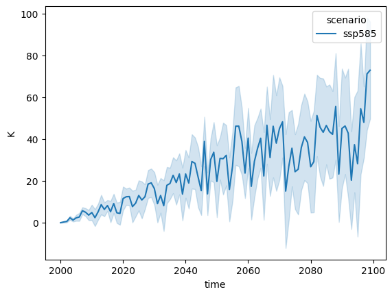
ScmRun.from_nc(OUTPUT_DIR / "out-ssp585-sparse.nc").filter(
    variable="Surface Temperature"
).line_plot()
For such a data set, since both run_id and paraset_id vary, both could be added as dimensions
in the file.
The one problem with this approach is that you get very sparse arrays because the data is written on a 100 x 30 x 90 (time points x paraset_id x run_id) grid but there’s only 90 timeseries so you end up with 180 timeseries worth of nans (although this is a relatively small problem because the netCDF files use compression to minismise the impact of the extra nan values).
xr.load_dataset(OUTPUT_DIR / "out-ssp585-sparse.nc")
<xarray.Dataset>
Dimensions:                          (time: 100, run_id: 30, paraset_id: 10)
Coordinates:
  * time                             (time) datetime64[ns] 2000-01-01 ... 209...
  * run_id                           (run_id) int64 60 61 62 63 ... 86 87 88 89
  * paraset_id                       (paraset_id) int64 0 1 2 3 4 5 6 7 8 9
Data variables:
    Surface_Temperature              (run_id, paraset_id, time) float64 0.0 ....
    Atmospheric_Concentrations__CO2  (run_id, paraset_id, time) float64 nan ....
    Radiative_Forcing                (run_id, paraset_id, time) float64 nan ....
Attributes:
    scmdata_metadata_scenario:  ssp585
    scmdata_metadata_model:     example
    scmdata_metadata_region:    World
    created_at:                 2024-01-29T07:18:02.481132
_scmdata_version: 1.0.0# Load all scenarios
run_append([ScmRun.from_nc(fname) for fname in OUTPUT_DIR.glob("out-ssp*-sparse.nc")])
<ScmRun (timeseries: 90, timepoints: 100)>
Time:
	Start: 2000-01-01T00:00:00
	End: 2099-01-01T00:00:00
Meta:
	      model  paraset_id region  run_id scenario   unit  \
	0   example           0  World      30   ssp370      K
	1   example           0  World      31   ssp370    ppm
	2   example           0  World      32   ssp370  W/m^2
	3   example           1  World      33   ssp370      K
	4   example           1  World      34   ssp370    ppm
	..      ...         ...    ...     ...      ...    ...
	85  example           8  World      85   ssp585    ppm
	86  example           8  World      86   ssp585  W/m^2
	87  example           9  World      87   ssp585      K
	88  example           9  World      88   ssp585    ppm
	89  example           9  World      89   ssp585  W/m^2

	                          variable
	0              Surface Temperature
	1   Atmospheric Concentrations|CO2
	2                Radiative Forcing
	3              Surface Temperature
	4   Atmospheric Concentrations|CO2
	..                             ...
	85  Atmospheric Concentrations|CO2
	86               Radiative Forcing
	87             Surface Temperature
	88  Atmospheric Concentrations|CO2
	89               Radiative Forcing

	[90 rows x 7 columns]
An alternative to the sparse arrays is to specify the variables in the extras attribute. If
possible, this adds the metadata to the netCDF file as an extra co-ordinate, which uses one of
the dimensions as it’s co-ordinate. If using one of the dimensions as a co-ordinate would not
specify the metadata uniquely, we add the extra as an additional co-ordinate, which itself has
co-ordinates of _id. This _id co-ordinate provides a unique mapping between the extra metadata
and the timeseries.
for sce_run in large_run.groupby("scenario"):
    sce = sce_run.get_unique_meta("scenario", True)
    sce_run.to_nc(
        OUTPUT_DIR / f"out-{sce}-extras.nc",
        dimensions=["run_id"],
        extras=["paraset_id"],
    )
/home/docs/checkouts/readthedocs.org/user_builds/scmdata/checkouts/stable/src/scmdata/_xarray.py:201: FutureWarning: Series.__getitem__ treating keys as positions is deprecated. In a future version, integer keys will always be treated as labels (consistent with DataFrame behavior). To access a value by position, use `ser.iloc[pos]`
  max_count = checker.groupby(col2).count().max()[0]
/home/docs/checkouts/readthedocs.org/user_builds/scmdata/checkouts/stable/src/scmdata/_xarray.py:236: FutureWarning: The previous implementation of stack is deprecated and will be removed in a future version of pandas. See the What's New notes for pandas 2.1.0 for details. Specify future_stack=True to adopt the new implementation and silence this warning.
  else timeseries.T.stack(dimensions)
paraset_id is uniquely defined by run_id so we don’t end up with an extra _id co-ordinate.
xr.load_dataset(OUTPUT_DIR / "out-ssp585-extras.nc")
<xarray.Dataset>
Dimensions:                          (time: 100, run_id: 30)
Coordinates:
  * time                             (time) datetime64[ns] 2000-01-01 ... 209...
  * run_id                           (run_id) int64 60 61 62 63 ... 86 87 88 89
    paraset_id                       (run_id) int64 0 0 0 1 1 1 ... 8 8 8 9 9 9
Data variables:
    Surface_Temperature              (run_id, time) float64 0.0 0.6824 ... nan
    Atmospheric_Concentrations__CO2  (run_id, time) float64 nan nan ... nan nan
    Radiative_Forcing                (run_id, time) float64 nan nan ... 9.579
Attributes:
    scmdata_metadata_scenario:  ssp585
    scmdata_metadata_model:     example
    scmdata_metadata_region:    World
    created_at:                 2024-01-29T07:18:03.360352
_scmdata_version: 1.0.0ScmRun.from_nc(OUTPUT_DIR / "out-ssp585-extras.nc").filter(
variable="Surface Temperature"
).line_plot()
If we use dimensions and extra such that our extra co-ordinates are not uniquely defined by the
regions, an _id dimension is automatically added to ensure we don’t lose any information.
large_run.to_nc(
    OUTPUT_DIR / "out-extras-sparse.nc",
    dimensions=["scenario"],
    extras=["paraset_id", "run_id"],
)
/home/docs/checkouts/readthedocs.org/user_builds/scmdata/checkouts/stable/src/scmdata/_xarray.py:201: FutureWarning: Series.__getitem__ treating keys as positions is deprecated. In a future version, integer keys will always be treated as labels (consistent with DataFrame behavior). To access a value by position, use `ser.iloc[pos]`
  max_count = checker.groupby(col2).count().max()[0]
/home/docs/checkouts/readthedocs.org/user_builds/scmdata/checkouts/stable/src/scmdata/_xarray.py:234: FutureWarning: The previous implementation of stack is deprecated and will be removed in a future version of pandas. See the What's New notes for pandas 2.1.0 for details. Specify future_stack=True to adopt the new implementation and silence this warning.
  timeseries.T.stack([*dimensions, "_id"])
xr.load_dataset(OUTPUT_DIR / "out-extras-sparse.nc")
<xarray.Dataset>
Dimensions:                          (time: 100, scenario: 3, _id: 90)
Coordinates:
  * time                             (time) datetime64[ns] 2000-01-01 ... 209...
  * scenario                         (scenario) <U6 'ssp119' 'ssp370' 'ssp585'
  * _id                              (_id) int64 0 1 2 3 4 5 ... 85 86 87 88 89
    paraset_id                       (_id) int64 0 0 0 1 1 1 2 ... 7 8 8 8 9 9 9
    run_id                           (_id) int64 0 1 2 3 4 5 ... 85 86 87 88 89
Data variables:
    Surface_Temperature              (scenario, time, _id) float64 0.0 ... nan
    Atmospheric_Concentrations__CO2  (scenario, time, _id) float64 nan ... nan
    Radiative_Forcing                (scenario, time, _id) float64 nan ... 9.579
Attributes:
    scmdata_metadata_model:   example
    scmdata_metadata_region:  World
    created_at:               2024-01-29T07:18:04.000759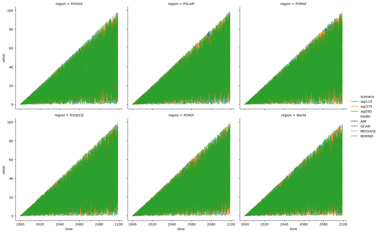
_scmdata_version: 1.0.0Multi-dimensional data
scmdata can also handle having more than one dimension. This can be especially helpful if you have output from a number of models (IAMs), scenarios, regions and runs.
multi_dimensional_run = []

for model in ["AIM", "GCAM", "MESSAGE", "REMIND"]:
    for sce in ["ssp119", "ssp370", "ssp585"]:
        for region in ["World", "R5LAM", "R5MAF", "R5ASIA", "R5OECD", "R5REF"]:
            multi_dimensional_run.extend(
                [
                    new_timeseries(
                        count=3,
                        model=model,
                        scenario=sce,
                        region=region,
                        variable=[
                            "Surface Temperature",
                            "Atmospheric Concentrations|CO2",
                            "Radiative Forcing",
                        ],
                        unit=["K", "ppm", "W/m^2"],
                        paraset_id=paraset_id,
                    )
                    for paraset_id in range(10)
                ]
            )

multi_dimensional_run = run_append(multi_dimensional_run)

multi_dimensional_run
<ScmRun (timeseries: 2160, timepoints: 100)>
Time:
	Start: 2000-01-01T00:00:00
	End: 2099-01-01T00:00:00
Meta:
	       model  paraset_id region scenario   unit  \
	0        AIM           0  World   ssp119      K
	1        AIM           0  World   ssp119    ppm
	2        AIM           0  World   ssp119  W/m^2
	3        AIM           1  World   ssp119      K
	4        AIM           1  World   ssp119    ppm
	...      ...         ...    ...      ...    ...
	2155  REMIND           8  R5REF   ssp585    ppm
	2156  REMIND           8  R5REF   ssp585  W/m^2
	2157  REMIND           9  R5REF   ssp585      K
	2158  REMIND           9  R5REF   ssp585    ppm
	2159  REMIND           9  R5REF   ssp585  W/m^2

	                            variable
	0                Surface Temperature
	1     Atmospheric Concentrations|CO2
	2                  Radiative Forcing
	3                Surface Temperature
	4     Atmospheric Concentrations|CO2
	...                              ...
	2155  Atmospheric Concentrations|CO2
	2156               Radiative Forcing
	2157             Surface Temperature
	2158  Atmospheric Concentrations|CO2
	2159               Radiative Forcing

	[2160 rows x 6 columns]
multi_dim_outfile = OUTPUT_DIR / "out-multi-dimensional.nc"
multi_dimensional_run.to_nc(
    multi_dim_outfile,
    dimensions=("region", "model", "scenario", "paraset_id"),
)
/home/docs/checkouts/readthedocs.org/user_builds/scmdata/checkouts/stable/src/scmdata/_xarray.py:236: FutureWarning: The previous implementation of stack is deprecated and will be removed in a future version of pandas. See the What's New notes for pandas 2.1.0 for details. Specify future_stack=True to adopt the new implementation and silence this warning.
  else timeseries.T.stack(dimensions)
xr.load_dataset(multi_dim_outfile)
<xarray.Dataset>
Dimensions:                          (time: 100, scenario: 3, region: 6,
                                      paraset_id: 10, model: 4)
Coordinates:
  * time                             (time) datetime64[ns] 2000-01-01 ... 209...
  * scenario                         (scenario) <U6 'ssp119' 'ssp370' 'ssp585'
  * region                           (region) <U6 'R5ASIA' 'R5LAM' ... 'World'
  * paraset_id                       (paraset_id) int64 0 1 2 3 4 5 6 7 8 9
  * model                            (model) <U7 'AIM' 'GCAM' 'MESSAGE' 'REMIND'
Data variables:
    Surface_Temperature              (region, model, scenario, paraset_id, time) float64 ...
    Atmospheric_Concentrations__CO2  (region, model, scenario, paraset_id, time) float64 ...
    Radiative_Forcing                (region, model, scenario, paraset_id, time) float64 ...
Attributes:
    created_at:        2024-01-29T07:18:09.510062
_scmdata_version: 1.0.0multi_dim_loaded_co2_conc = ScmRun.from_nc(multi_dim_outfile).filter(
variable="Atmospheric Concentrations|CO2"
)
seaborn_df = multi_dim_loaded_co2_conc.long_data()
seaborn_df.head()
| model | paraset_id | region | scenario | unit | variable | time | value | |
|---|---|---|---|---|---|---|---|---|
| 0 | AIM | 0 | R5ASIA | ssp119 | ppm | Atmospheric Concentrations|CO2 | 2000-01-01 | 0.000000 |
| 1 | AIM | 0 | R5ASIA | ssp119 | ppm | Atmospheric Concentrations|CO2 | 2001-01-01 | 0.730551 |
| 2 | AIM | 0 | R5ASIA | ssp119 | ppm | Atmospheric Concentrations|CO2 | 2002-01-01 | 0.142061 |
| 3 | AIM | 0 | R5ASIA | ssp119 | ppm | Atmospheric Concentrations|CO2 | 2003-01-01 | 2.977609 |
| 4 | AIM | 0 | R5ASIA | ssp119 | ppm | Atmospheric Concentrations|CO2 | 2004-01-01 | 0.785949 |
sns.relplot(
    data=seaborn_df,
    x="time",
    y="value",
    units="paraset_id",
    estimator=None,
    hue="scenario",
    style="model",
    col="region",
    col_wrap=3,
    kind="line",
)
<seaborn.axisgrid.FacetGrid at 0x7f353ebbc490>