xarray compatibility

scmdata allows datat to be exported to xarray. This makes it easy to use xarray’s many helpful features, most of which are not natively provided in scmdata.

import numpy as np

from scmdata import ScmRun

/home/docs/checkouts/readthedocs.org/user_builds/scmdata/checkouts/stable/src/scmdata/database/_database.py:9: TqdmWarning: IProgress not found. Please update jupyter and ipywidgets. See https://ipywidgets.readthedocs.io/en/stable/user_install.html
  import tqdm.autonotebook as tqdman

def get_data(years, n_ensemble_members, end_val, rand_pct):
    """
    Get sample data
    """
    return (np.arange(years.shape[0]) / years.shape[0] * end_val)[:, np.newaxis] * (
        rand_pct * np.random.random((years.shape[0], n_ensemble_members)) + 1
    )

years = np.arange(1750, 2500 + 1)
variables = ["gsat", "gmst"]
n_variables = len(variables)
n_ensemble_members = 100


start = ScmRun(
    np.hstack(
        [
            get_data(years, n_ensemble_members, 5.5, 0.1),
            get_data(years, n_ensemble_members, 6.0, 0.05),
        ]
    ),
    index=years,
    columns={
        "model": "a_model",
        "scenario": "a_scenario",
        "variable": [v for v in variables for i in range(n_ensemble_members)],
        "region": "World",
        "unit": "K",
        "ensemble_member": [i for v in variables for i in range(n_ensemble_members)],
    },
)
start

<ScmRun (timeseries: 200, timepoints: 751)>
Time:
	Start: 1750-01-01T00:00:00
	End: 2500-01-01T00:00:00
Meta:
	     ensemble_member    model region    scenario unit variable
	0                  0  a_model  World  a_scenario    K     gsat
	1                  1  a_model  World  a_scenario    K     gsat
	2                  2  a_model  World  a_scenario    K     gsat
	3                  3  a_model  World  a_scenario    K     gsat
	4                  4  a_model  World  a_scenario    K     gsat
	..               ...      ...    ...         ...  ...      ...
	195               95  a_model  World  a_scenario    K     gmst
	196               96  a_model  World  a_scenario    K     gmst
	197               97  a_model  World  a_scenario    K     gmst
	198               98  a_model  World  a_scenario    K     gmst
	199               99  a_model  World  a_scenario    K     gmst
	
	[200 rows x 6 columns]

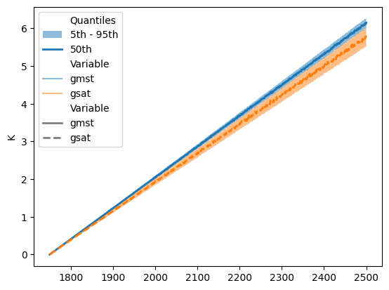
The usual scmdata methods are of course available.

start.plumeplot(
    quantile_over="ensemble_member", hue_var="variable", hue_label="Variable"
)

/home/docs/checkouts/readthedocs.org/user_builds/scmdata/checkouts/stable/src/scmdata/run.py:197: PerformanceWarning: DataFrame is highly fragmented.  This is usually the result of calling `frame.insert` many times, which has poor performance.  Consider joining all columns at once using pd.concat(axis=1) instead. To get a de-fragmented frame, use `newframe = frame.copy()`
  df.reset_index(inplace=True)
/home/docs/checkouts/readthedocs.org/user_builds/scmdata/checkouts/stable/src/scmdata/run.py:197: PerformanceWarning: DataFrame is highly fragmented.  This is usually the result of calling `frame.insert` many times, which has poor performance.  Consider joining all columns at once using pd.concat(axis=1) instead. To get a de-fragmented frame, use `newframe = frame.copy()`
  df.reset_index(inplace=True)
/home/docs/checkouts/readthedocs.org/user_builds/scmdata/checkouts/stable/src/scmdata/run.py:197: PerformanceWarning: DataFrame is highly fragmented.  This is usually the result of calling `frame.insert` many times, which has poor performance.  Consider joining all columns at once using pd.concat(axis=1) instead. To get a de-fragmented frame, use `newframe = frame.copy()`
  df.reset_index(inplace=True)
/home/docs/checkouts/readthedocs.org/user_builds/scmdata/checkouts/stable/src/scmdata/run.py:197: PerformanceWarning: DataFrame is highly fragmented.  This is usually the result of calling `frame.insert` many times, which has poor performance.  Consider joining all columns at once using pd.concat(axis=1) instead. To get a de-fragmented frame, use `newframe = frame.copy()`
  df.reset_index(inplace=True)
/home/docs/checkouts/readthedocs.org/user_builds/scmdata/checkouts/stable/src/scmdata/run.py:197: PerformanceWarning: DataFrame is highly fragmented.  This is usually the result of calling `frame.insert` many times, which has poor performance.  Consider joining all columns at once using pd.concat(axis=1) instead. To get a de-fragmented frame, use `newframe = frame.copy()`
  df.reset_index(inplace=True)
/home/docs/checkouts/readthedocs.org/user_builds/scmdata/checkouts/stable/src/scmdata/run.py:197: PerformanceWarning: DataFrame is highly fragmented.  This is usually the result of calling `frame.insert` many times, which has poor performance.  Consider joining all columns at once using pd.concat(axis=1) instead. To get a de-fragmented frame, use `newframe = frame.copy()`
  df.reset_index(inplace=True)

(<Axes: ylabel='K'>,
 [<matplotlib.patches.Patch at 0x7f9278342d00>,
  <matplotlib.collections.PolyCollection at 0x7f927833ab80>,
  <matplotlib.lines.Line2D at 0x7f9278158eb0>,
  <matplotlib.patches.Patch at 0x7f92ac050760>,
  <matplotlib.lines.Line2D at 0x7f92846e1580>,
  <matplotlib.lines.Line2D at 0x7f92836cedf0>,
  <matplotlib.patches.Patch at 0x7f92ac050190>,
  <matplotlib.lines.Line2D at 0x7f92836da100>,
  <matplotlib.lines.Line2D at 0x7f92836da0a0>])

However, we can cast to an xarray DataSet and then all the xarray methods become available too.

xr_ds = start.to_xarray(dimensions=("ensemble_member",))
xr_ds

/home/docs/checkouts/readthedocs.org/user_builds/scmdata/checkouts/stable/src/scmdata/_xarray.py:236: FutureWarning: The previous implementation of stack is deprecated and will be removed in a future version of pandas. See the What's New notes for pandas 2.1.0 for details. Specify future_stack=True to adopt the new implementation and silence this warning.
  else timeseries.T.stack(dimensions)

<xarray.Dataset>
Dimensions:          (time: 751, ensemble_member: 100)
Coordinates:
  * time             (time) object 1750-01-01 00:00:00 ... 2500-01-01 00:00:00
  * ensemble_member  (ensemble_member) int64 0 1 2 3 4 5 6 ... 94 95 96 97 98 99
Data variables:
    gsat             (ensemble_member, time) float64 0.0 0.007884 ... 5.881
    gmst             (ensemble_member, time) float64 0.0 0.008282 ... 6.227
Attributes:
    scmdata_metadata_region:    World
    scmdata_metadata_model:     a_model
    scmdata_metadata_scenario:  a_scenario

xarray.Dataset

• Dimensions:
  • time: 751
  • ensemble_member: 100
• Coordinates: (2)
  • time
    (time)
    object
    1750-01-01 00:00:00 ... 2500-01-...

    array([cftime.DatetimeGregorian(1750, 1, 1, 0, 0, 0, 0, has_year_zero=False),
           cftime.DatetimeGregorian(1751, 1, 1, 0, 0, 0, 0, has_year_zero=False),
           cftime.DatetimeGregorian(1752, 1, 1, 0, 0, 0, 0, has_year_zero=False),
           ...,
           cftime.DatetimeGregorian(2498, 1, 1, 0, 0, 0, 0, has_year_zero=False),
           cftime.DatetimeGregorian(2499, 1, 1, 0, 0, 0, 0, has_year_zero=False),
           cftime.DatetimeGregorian(2500, 1, 1, 0, 0, 0, 0, has_year_zero=False)],
          dtype=object)

  • ensemble_member
    (ensemble_member)
    int64
    0 1 2 3 4 5 6 ... 94 95 96 97 98 99

    array([ 0,  1,  2,  3,  4,  5,  6,  7,  8,  9, 10, 11, 12, 13, 14, 15, 16, 17,
           18, 19, 20, 21, 22, 23, 24, 25, 26, 27, 28, 29, 30, 31, 32, 33, 34, 35,
           36, 37, 38, 39, 40, 41, 42, 43, 44, 45, 46, 47, 48, 49, 50, 51, 52, 53,
           54, 55, 56, 57, 58, 59, 60, 61, 62, 63, 64, 65, 66, 67, 68, 69, 70, 71,
           72, 73, 74, 75, 76, 77, 78, 79, 80, 81, 82, 83, 84, 85, 86, 87, 88, 89,
           90, 91, 92, 93, 94, 95, 96, 97, 98, 99])

• Data variables: (2)
  • gsat
    (ensemble_member, time)
    float64
    0.0 0.007884 ... 5.711 5.881

    units :

    K

    array([[0.        , 0.00788388, 0.01487158, ..., 5.8450021 , 5.72467187,
            5.72726153],
           [0.        , 0.00797886, 0.01475376, ..., 5.99291185, 5.6938214 ,
            5.74488585],
           [0.        , 0.00769549, 0.01561708, ..., 5.88667401, 5.79525945,
            5.7664412 ],
           ...,
           [0.        , 0.00762947, 0.01599446, ..., 5.68111068, 5.87512087,
            5.63480056],
           [0.        , 0.00740279, 0.01570517, ..., 5.71870567, 5.74311884,
            5.74640267],
           [0.        , 0.0077345 , 0.01591274, ..., 5.98104471, 5.71096204,
            5.88112551]])

  • gmst
    (ensemble_member, time)
    float64
    0.0 0.008282 ... 6.177 6.227

    units :

    K

    array([[0.        , 0.00828181, 0.01645457, ..., 6.16541091, 6.00697132,
            6.14631791],
           [0.        , 0.0080324 , 0.01601351, ..., 6.0171424 , 6.13030082,
            6.1948832 ],
           [0.        , 0.00809838, 0.01625457, ..., 6.2637564 , 6.13074318,
            6.11882818],
           ...,
           [0.        , 0.00818538, 0.01677099, ..., 6.21610244, 6.01467206,
            6.02437685],
           [0.        , 0.00822822, 0.01666612, ..., 5.99720127, 6.22522985,
            6.21697571],
           [0.        , 0.00826254, 0.01599292, ..., 6.13809839, 6.1767361 ,
            6.22665719]])

• Indexes: (2)
  • time
    PandasIndex

    PandasIndex(CFTimeIndex([1750-01-01 00:00:00, 1751-01-01 00:00:00, 1752-01-01 00:00:00,
                 1753-01-01 00:00:00, 1754-01-01 00:00:00, 1755-01-01 00:00:00,
                 1756-01-01 00:00:00, 1757-01-01 00:00:00, 1758-01-01 00:00:00,
                 1759-01-01 00:00:00,
                 ...
                 2491-01-01 00:00:00, 2492-01-01 00:00:00, 2493-01-01 00:00:00,
                 2494-01-01 00:00:00, 2495-01-01 00:00:00, 2496-01-01 00:00:00,
                 2497-01-01 00:00:00, 2498-01-01 00:00:00, 2499-01-01 00:00:00,
                 2500-01-01 00:00:00],
                dtype='object', length=751, calendar='standard', freq='YS-JAN'))

  • ensemble_member
    PandasIndex

    PandasIndex(Index([ 0,  1,  2,  3,  4,  5,  6,  7,  8,  9, 10, 11, 12, 13, 14, 15, 16, 17,
           18, 19, 20, 21, 22, 23, 24, 25, 26, 27, 28, 29, 30, 31, 32, 33, 34, 35,
           36, 37, 38, 39, 40, 41, 42, 43, 44, 45, 46, 47, 48, 49, 50, 51, 52, 53,
           54, 55, 56, 57, 58, 59, 60, 61, 62, 63, 64, 65, 66, 67, 68, 69, 70, 71,
           72, 73, 74, 75, 76, 77, 78, 79, 80, 81, 82, 83, 84, 85, 86, 87, 88, 89,
           90, 91, 92, 93, 94, 95, 96, 97, 98, 99],
          dtype='int64', name='ensemble_member'))

• Attributes: (3)

  scmdata_metadata_region :

  World

  scmdata_metadata_model :

  a_model

  scmdata_metadata_scenario :

  a_scenario

For example, calculating statistics.

xr_ds.median(dim="ensemble_member")

<xarray.Dataset>
Dimensions:  (time: 751)
Coordinates:
  * time     (time) object 1750-01-01 00:00:00 ... 2500-01-01 00:00:00
Data variables:
    gsat     (time) float64 0.0 0.007716 0.01544 0.02297 ... 5.748 5.789 5.775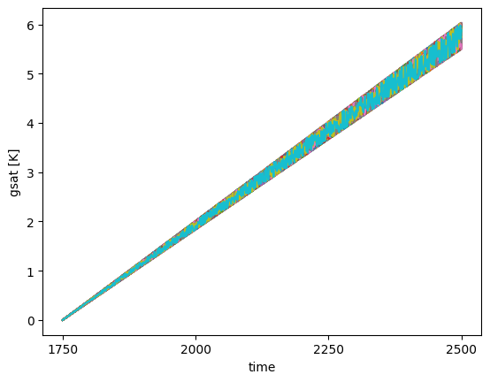
    gmst     (time) float64 0.0 0.008173 0.01646 0.02462 ... 6.135 6.113 6.151

xarray.Dataset

• Dimensions:
  • time: 751
• Coordinates: (1)
  • time
    (time)
    object
    1750-01-01 00:00:00 ... 2500-01-...

    array([cftime.DatetimeGregorian(1750, 1, 1, 0, 0, 0, 0, has_year_zero=False),
           cftime.DatetimeGregorian(1751, 1, 1, 0, 0, 0, 0, has_year_zero=False),
           cftime.DatetimeGregorian(1752, 1, 1, 0, 0, 0, 0, has_year_zero=False),
           ...,
           cftime.DatetimeGregorian(2498, 1, 1, 0, 0, 0, 0, has_year_zero=False),
           cftime.DatetimeGregorian(2499, 1, 1, 0, 0, 0, 0, has_year_zero=False),
           cftime.DatetimeGregorian(2500, 1, 1, 0, 0, 0, 0, has_year_zero=False)],
          dtype=object)

• Data variables: (2)
  • gsat
    (time)
    float64
    0.0 0.007716 ... 5.789 5.775

    array([0.        , 0.00771645, 0.01544448, 0.02296606, 0.03081341,
           0.03833551, 0.04570844, 0.05402774, 0.06175181, 0.06913292,
           0.07704609, 0.0840496 , 0.09192515, 0.09951401, 0.10820434,
           0.11596456, 0.12365671, 0.1301869 , 0.13819346, 0.14751522,
           0.15451262, 0.16001477, 0.16974128, 0.17630603, 0.18351922,
           0.19173147, 0.20067586, 0.2081953 , 0.21571302, 0.22301354,
           0.23050131, 0.23899925, 0.2458271 , 0.25299338, 0.26095025,
           0.27184527, 0.27630751, 0.28428007, 0.29280657, 0.30069386,
           0.30830934, 0.31777874, 0.32389297, 0.32948952, 0.33711674,
           0.34673331, 0.35577914, 0.3629739 , 0.36840446, 0.37505257,
           0.38164519, 0.3951427 , 0.39956392, 0.4071688 , 0.41247152,
           0.42225913, 0.43064733, 0.43906408, 0.44583572, 0.45168998,
           0.46320845, 0.47015728, 0.47960182, 0.48083979, 0.49465052,
           0.50153262, 0.50710574, 0.51757363, 0.52359132, 0.53174307,
           0.53904933, 0.54829104, 0.55868832, 0.55910803, 0.56757009,
           0.57766682, 0.58834528, 0.59047333, 0.59364458, 0.60791655,
           0.61373314, 0.62307496, 0.63264181, 0.63663933, 0.65365014,
           0.65249261, 0.66115333, 0.66812036, 0.66800707, 0.68501053,
           0.68738015, 0.69735877, 0.70665518, 0.71585722, 0.7198166 ,
           0.72078615, 0.73370747, 0.74846232, 0.74854805, 0.75712475,
    ...
           5.06615784, 5.03786939, 5.03881562, 5.07829931, 5.11154682,
           5.05826028, 5.08889494, 5.08871907, 5.09319942, 5.09013165,
           5.13210212, 5.13157039, 5.11536062, 5.13350554, 5.13268553,
           5.13840841, 5.12113616, 5.18436038, 5.18683362, 5.17735082,
           5.21436627, 5.20216163, 5.19991126, 5.17290804, 5.23661507,
           5.26458483, 5.24562329, 5.28533873, 5.27745856, 5.22444971,
           5.27528544, 5.27910698, 5.27500713, 5.28248886, 5.31209709,
           5.32505419, 5.36270913, 5.32915402, 5.31055581, 5.32917018,
           5.33282113, 5.36224747, 5.34282856, 5.36416786, 5.38366579,
           5.41259532, 5.37494845, 5.41125102, 5.44027689, 5.36471416,
           5.43862285, 5.40884866, 5.42103974, 5.43695246, 5.45734525,
           5.4279737 , 5.46457406, 5.46402448, 5.49478823, 5.51233755,
           5.49470889, 5.56752307, 5.48732055, 5.50739626, 5.56058787,
           5.51553938, 5.56627395, 5.52813968, 5.56326134, 5.55694297,
           5.55730269, 5.58095179, 5.58793234, 5.62812331, 5.6438767 ,
           5.60625412, 5.64050707, 5.65062288, 5.62518758, 5.61829729,
           5.63400468, 5.68298684, 5.68105816, 5.64106261, 5.64710089,
           5.64219444, 5.71971515, 5.68679176, 5.6878916 , 5.75187917,
           5.73282013, 5.69730297, 5.76776442, 5.74827527, 5.78862945,
           5.774752  ])

  • gmst
    (time)
    float64
    0.0 0.008173 ... 6.113 6.151

    array([0.        , 0.00817283, 0.01645929, 0.02461525, 0.03271932,
           0.04078525, 0.04895776, 0.05743444, 0.06529063, 0.07366855,
           0.08144891, 0.08979245, 0.09832628, 0.10652199, 0.11475829,
           0.12309583, 0.13052603, 0.13920805, 0.1469818 , 0.15514574,
           0.16366934, 0.17261482, 0.18047466, 0.1880569 , 0.19618389,
           0.20456748, 0.21300344, 0.22102909, 0.22846559, 0.23720892,
           0.24637716, 0.25446813, 0.26310592, 0.26989454, 0.27875882,
           0.28695888, 0.29438615, 0.30337414, 0.31159591, 0.32052346,
           0.32680407, 0.33574192, 0.34407088, 0.35224245, 0.36046511,
           0.36783837, 0.37772907, 0.38520916, 0.39320126, 0.40112678,
           0.41043783, 0.41757876, 0.42552602, 0.43406375, 0.44134774,
           0.45063283, 0.45881189, 0.46801037, 0.4757526 , 0.48132915,
           0.49332801, 0.4992933 , 0.50785452, 0.51381189, 0.52259298,
           0.53132117, 0.54050098, 0.55050256, 0.55771367, 0.5648569 ,
           0.57278832, 0.58080992, 0.5914616 , 0.5977231 , 0.60458097,
           0.61272061, 0.62230659, 0.63112343, 0.63895765, 0.64999521,
           0.65452723, 0.66459048, 0.67112495, 0.68092493, 0.68535466,
           0.69406883, 0.70372722, 0.7122931 , 0.72365864, 0.72720467,
           0.73506719, 0.74636873, 0.7549069 , 0.76119163, 0.76997302,
           0.77480551, 0.78851967, 0.79304032, 0.80572732, 0.80655934,
    ...
           5.36157392, 5.36835343, 5.38543083, 5.38818159, 5.40002587,
           5.38706692, 5.40381899, 5.39074662, 5.4205747 , 5.42573074,
           5.42436188, 5.46266671, 5.4673254 , 5.45251151, 5.46087637,
           5.49254552, 5.5104248 , 5.49306714, 5.51452527, 5.53062863,
           5.56123602, 5.54903012, 5.56216675, 5.54599207, 5.54435605,
           5.58720392, 5.59050787, 5.580553  , 5.6018567 , 5.61060093,
           5.5899282 , 5.6026137 , 5.59685135, 5.6320331 , 5.634327  ,
           5.65532997, 5.6486992 , 5.6771206 , 5.67515697, 5.67899711,
           5.70623477, 5.69914297, 5.72726188, 5.73446822, 5.73496156,
           5.74705811, 5.73800013, 5.74121591, 5.7541866 , 5.7626406 ,
           5.77563707, 5.77624658, 5.75811242, 5.81288017, 5.81211155,
           5.81731096, 5.81171746, 5.85204517, 5.85380478, 5.87961591,
           5.84712988, 5.87046755, 5.88106781, 5.86275152, 5.89074906,
           5.89814439, 5.87719913, 5.93350186, 5.92256026, 5.94923611,
           5.94717488, 5.94846016, 5.93630454, 5.96813319, 5.98633065,
           5.9582268 , 5.99920519, 5.9849397 , 5.99037385, 6.01696532,
           5.99171445, 6.0206863 , 6.02621778, 6.04537675, 6.08077713,
           6.06897847, 6.07188628, 6.08190637, 6.06736667, 6.0948821 ,
           6.08838665, 6.1196844 , 6.10025325, 6.13504241, 6.11314084,
           6.15086412])

• Indexes: (1)
  • time
    PandasIndex

    PandasIndex(CFTimeIndex([1750-01-01 00:00:00, 1751-01-01 00:00:00, 1752-01-01 00:00:00,
                 1753-01-01 00:00:00, 1754-01-01 00:00:00, 1755-01-01 00:00:00,
                 1756-01-01 00:00:00, 1757-01-01 00:00:00, 1758-01-01 00:00:00,
                 1759-01-01 00:00:00,
                 ...
                 2491-01-01 00:00:00, 2492-01-01 00:00:00, 2493-01-01 00:00:00,
                 2494-01-01 00:00:00, 2495-01-01 00:00:00, 2496-01-01 00:00:00,
                 2497-01-01 00:00:00, 2498-01-01 00:00:00, 2499-01-01 00:00:00,
                 2500-01-01 00:00:00],
                dtype='object', length=751, calendar='standard', freq='YS-JAN'))

• Attributes: (0)

Plotting timeseries.

xr_ds["gsat"].plot.line(hue="ensemble_member", add_legend=False)

[<matplotlib.lines.Line2D at 0x7f927582c640>,
 <matplotlib.lines.Line2D at 0x7f927577f6d0>,
 <matplotlib.lines.Line2D at 0x7f927577f7f0>,
 <matplotlib.lines.Line2D at 0x7f927577f9a0>,
 <matplotlib.lines.Line2D at 0x7f927577fa90>,
 <matplotlib.lines.Line2D at 0x7f927577fb80>,
 <matplotlib.lines.Line2D at 0x7f927577fc70>,
 <matplotlib.lines.Line2D at 0x7f927577fd60>,
 <matplotlib.lines.Line2D at 0x7f927577fe50>,
 <matplotlib.lines.Line2D at 0x7f927577ff40>,
 <matplotlib.lines.Line2D at 0x7f9275791070>,
 <matplotlib.lines.Line2D at 0x7f9275791190>,
 <matplotlib.lines.Line2D at 0x7f9275791280>,
 <matplotlib.lines.Line2D at 0x7f9275791370>,
 <matplotlib.lines.Line2D at 0x7f9275791460>,
 <matplotlib.lines.Line2D at 0x7f9275791550>,
 <matplotlib.lines.Line2D at 0x7f9275791640>,
 <matplotlib.lines.Line2D at 0x7f9275791730>,
 <matplotlib.lines.Line2D at 0x7f9275791820>,
 <matplotlib.lines.Line2D at 0x7f9275791910>,
 <matplotlib.lines.Line2D at 0x7f9275791a00>,
 <matplotlib.lines.Line2D at 0x7f9275791af0>,
 <matplotlib.lines.Line2D at 0x7f9275791be0>,
 <matplotlib.lines.Line2D at 0x7f9275791cd0>,
 <matplotlib.lines.Line2D at 0x7f9275791dc0>,
 <matplotlib.lines.Line2D at 0x7f9275791eb0>,
 <matplotlib.lines.Line2D at 0x7f9275791fa0>,
 <matplotlib.lines.Line2D at 0x7f92757ac5b0>,
 <matplotlib.lines.Line2D at 0x7f92757ac910>,
 <matplotlib.lines.Line2D at 0x7f92757aca00>,
 <matplotlib.lines.Line2D at 0x7f92757acaf0>,
 <matplotlib.lines.Line2D at 0x7f92757acbe0>,
 <matplotlib.lines.Line2D at 0x7f92757accd0>,
 <matplotlib.lines.Line2D at 0x7f92757acdc0>,
 <matplotlib.lines.Line2D at 0x7f92757aceb0>,
 <matplotlib.lines.Line2D at 0x7f92757acfa0>,
 <matplotlib.lines.Line2D at 0x7f92757ac4c0>,
 <matplotlib.lines.Line2D at 0x7f92757ac370>,
 <matplotlib.lines.Line2D at 0x7f92757ac250>,
 <matplotlib.lines.Line2D at 0x7f92757ac160>,
 <matplotlib.lines.Line2D at 0x7f9275794070>,
 <matplotlib.lines.Line2D at 0x7f9275794160>,
 <matplotlib.lines.Line2D at 0x7f9275794250>,
 <matplotlib.lines.Line2D at 0x7f9275794eb0>,
 <matplotlib.lines.Line2D at 0x7f9275794dc0>,
 <matplotlib.lines.Line2D at 0x7f9275794cd0>,
 <matplotlib.lines.Line2D at 0x7f9275794be0>,
 <matplotlib.lines.Line2D at 0x7f9275794af0>,
 <matplotlib.lines.Line2D at 0x7f9275794a00>,
 <matplotlib.lines.Line2D at 0x7f9275794910>,
 <matplotlib.lines.Line2D at 0x7f9275794820>,
 <matplotlib.lines.Line2D at 0x7f9275794730>,
 <matplotlib.lines.Line2D at 0x7f9275794640>,
 <matplotlib.lines.Line2D at 0x7f9275794550>,
 <matplotlib.lines.Line2D at 0x7f9275794460>,
 <matplotlib.lines.Line2D at 0x7f9275794370>,
 <matplotlib.lines.Line2D at 0x7f9275794280>,
 <matplotlib.lines.Line2D at 0x7f92757dddf0>,
 <matplotlib.lines.Line2D at 0x7f92757ddf10>,
 <matplotlib.lines.Line2D at 0x7f927579bfa0>,
 <matplotlib.lines.Line2D at 0x7f92757daeb0>,
 <matplotlib.lines.Line2D at 0x7f92757daee0>,
 <matplotlib.lines.Line2D at 0x7f92757c2040>,
 <matplotlib.lines.Line2D at 0x7f927582cf70>,
 <matplotlib.lines.Line2D at 0x7f927579bd30>,
 <matplotlib.lines.Line2D at 0x7f927579bc40>,
 <matplotlib.lines.Line2D at 0x7f927579bb50>,
 <matplotlib.lines.Line2D at 0x7f927579ba60>,
 <matplotlib.lines.Line2D at 0x7f927579b970>,
 <matplotlib.lines.Line2D at 0x7f927579b880>,
 <matplotlib.lines.Line2D at 0x7f927579b790>,
 <matplotlib.lines.Line2D at 0x7f927579b6a0>,
 <matplotlib.lines.Line2D at 0x7f927579b5b0>,
 <matplotlib.lines.Line2D at 0x7f927579b4c0>,
 <matplotlib.lines.Line2D at 0x7f927579b3d0>,
 <matplotlib.lines.Line2D at 0x7f927579b2e0>,
 <matplotlib.lines.Line2D at 0x7f927579b1f0>,
 <matplotlib.lines.Line2D at 0x7f927579b100>,
 <matplotlib.lines.Line2D at 0x7f927578cfd0>,
 <matplotlib.lines.Line2D at 0x7f927578cee0>,
 <matplotlib.lines.Line2D at 0x7f927578cdf0>,
 <matplotlib.lines.Line2D at 0x7f927578cd00>,
 <matplotlib.lines.Line2D at 0x7f927578cc10>,
 <matplotlib.lines.Line2D at 0x7f927578cb20>,
 <matplotlib.lines.Line2D at 0x7f927578ca30>,
 <matplotlib.lines.Line2D at 0x7f927578c940>,
 <matplotlib.lines.Line2D at 0x7f927578c850>,
 <matplotlib.lines.Line2D at 0x7f927578c760>,
 <matplotlib.lines.Line2D at 0x7f927578c670>,
 <matplotlib.lines.Line2D at 0x7f927578c580>,
 <matplotlib.lines.Line2D at 0x7f927578c490>,
 <matplotlib.lines.Line2D at 0x7f927578c3a0>,
 <matplotlib.lines.Line2D at 0x7f927578c2b0>,
 <matplotlib.lines.Line2D at 0x7f927578c1c0>,
 <matplotlib.lines.Line2D at 0x7f927578c0d0>,
 <matplotlib.lines.Line2D at 0x7f9275784fa0>,
 <matplotlib.lines.Line2D at 0x7f9275784eb0>,
 <matplotlib.lines.Line2D at 0x7f9275784dc0>,
 <matplotlib.lines.Line2D at 0x7f9275784cd0>,
 <matplotlib.lines.Line2D at 0x7f9275784be0>]

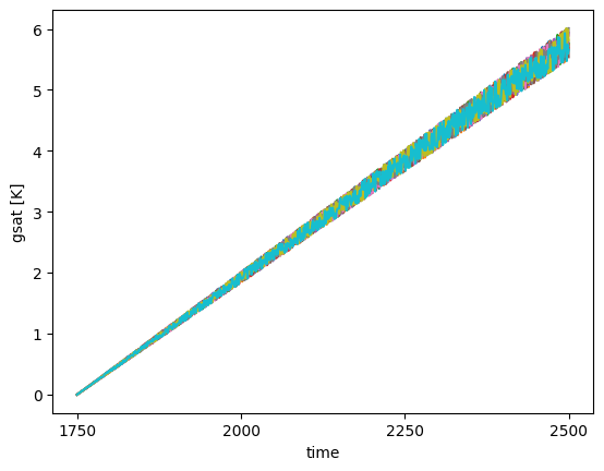
Selecting and plotting timeseries.

xr_ds["gsat"].sel(ensemble_member=range(10)).plot.line(
    hue="ensemble_member", add_legend=False
)

[<matplotlib.lines.Line2D at 0x7f92756aae80>,
 <matplotlib.lines.Line2D at 0x7f9275662400>,
 <matplotlib.lines.Line2D at 0x7f9275662550>,
 <matplotlib.lines.Line2D at 0x7f92756626d0>,
 <matplotlib.lines.Line2D at 0x7f92756627c0>,
 <matplotlib.lines.Line2D at 0x7f92756628b0>,
 <matplotlib.lines.Line2D at 0x7f92756629a0>,
 <matplotlib.lines.Line2D at 0x7f9275662a90>,
 <matplotlib.lines.Line2D at 0x7f9275662b80>,
 <matplotlib.lines.Line2D at 0x7f9275662c70>]

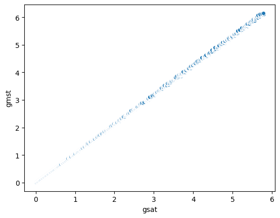
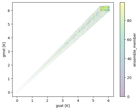
Scatter plots.

xr_ds.plot.scatter(x="gsat", y="gmst", hue="ensemble_member", alpha=0.3)

<matplotlib.collections.PathCollection at 0x7f92755b3be0>

Or combinations of calculations and plots.

xr_ds.median(dim="ensemble_member").plot.scatter(x="gsat", y="gmst")

<matplotlib.collections.PathCollection at 0x7f92754dbb50>