Time operations

Time operations are notoriously difficult. In this notebook we go through some of scmdata’s time operation capabilities.

Imports

import datetime as dt
import traceback

import matplotlib.pyplot as plt
from pandas.plotting import register_matplotlib_converters

import scmdata.errors
import scmdata.time
from scmdata import ScmRun, run_append

register_matplotlib_converters()

/tmp/ipykernel_914/1092330876.py:5: DeprecationWarning: 
Pyarrow will become a required dependency of pandas in the next major release of pandas (pandas 3.0),
(to allow more performant data types, such as the Arrow string type, and better interoperability with other libraries)
but was not found to be installed on your system.
If this would cause problems for you,
please provide us feedback at https://github.com/pandas-dev/pandas/issues/54466
        
  from pandas.plotting import register_matplotlib_converters
/home/docs/checkouts/readthedocs.org/user_builds/scmdata/checkouts/stable/src/scmdata/database/_database.py:9: TqdmWarning: IProgress not found. Please update jupyter and ipywidgets. See https://ipywidgets.readthedocs.io/en/stable/user_install.html
  import tqdm.autonotebook as tqdman

Data

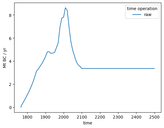
Here we use the RCP26 emissions data. This originally came from http://www.pik-potsdam.de/~mmalte/rcps/ and has since been re-written into a format which can be read by scmdata using the pymagicc library. We are not currently planning on importing Pymagicc’s readers into scmdata by default, please raise an issue here if you would like us to consider doing so.

var_to_plot = "Emissions|BC"

rcp26 = ScmRun("rcp26_emissions.csv")
rcp26["time operation"] = "raw"

rcp26.filter(variable=var_to_plot).lineplot(hue="time operation")

<Axes: xlabel='time', ylabel='Mt BC / yr'>

../_images/ac5dbe87f2fb78978d5a89f878a70462da578911d35034c9b51d5f780e12e685.png

For illustrative purposes, we shift the time points of the raw data before moving on.

rcp26["time"] = rcp26["time"].map(lambda x: dt.datetime(x.year, 3, 17))
rcp26 = ScmRun(rcp26)
rcp26.head()

					time	1765-03-17 00:00:00	1766-03-17 00:00:00	1767-03-17 00:00:00	1768-03-17 00:00:00	1769-03-17 00:00:00	1770-03-17 00:00:00	1771-03-17 00:00:00	1772-03-17 00:00:00	1773-03-17 00:00:00	1774-03-17 00:00:00	...	2491-03-17 00:00:00	2492-03-17 00:00:00	2493-03-17 00:00:00	2494-03-17 00:00:00	2495-03-17 00:00:00	2496-03-17 00:00:00	2497-03-17 00:00:00	2498-03-17 00:00:00	2499-03-17 00:00:00	2500-03-17 00:00:00
model	region	scenario	time operation	unit	variable
IMAGE	World	RCP26	raw	Mt BC / yr	Emissions\|BC	0.000000	0.106998	0.133383	0.159847	0.186393	0.213024	0.239742	0.266550	0.293450	0.320446	...	3.3578	3.3578	3.3578	3.3578	3.3578	3.3578	3.3578	3.3578	3.3578	3.3578
				kt C2F6 / yr	Emissions\|C2F6	0.000000	0.000000	0.000000	0.000000	0.000000	0.000000	0.000000	0.000000	0.000000	0.000000	...	0.0857	0.0857	0.0857	0.0857	0.0857	0.0857	0.0857	0.0857	0.0857	0.0857
				kt C6F14 / yr	Emissions\|C6F14	0.000000	0.000000	0.000000	0.000000	0.000000	0.000000	0.000000	0.000000	0.000000	0.000000	...	0.0887	0.0887	0.0887	0.0887	0.0887	0.0887	0.0887	0.0887	0.0887	0.0887
				kt CCl4 / yr	Emissions\|CCl4	0.000000	0.000000	0.000000	0.000000	0.000000	0.000000	0.000000	0.000000	0.000000	0.000000	...	0.0000	0.0000	0.0000	0.0000	0.0000	0.0000	0.0000	0.0000	0.0000	0.0000
				kt CF4 / yr	Emissions\|CF4	0.010763	0.010752	0.010748	0.010744	0.010740	0.010736	0.010731	0.010727	0.010723	0.010719	...	1.0920	1.0920	1.0920	1.0920	1.0920	1.0920	1.0920	1.0920	1.0920	1.0920

5 rows × 736 columns

Resampling

The first method to consider is resample. This allows us to resample a dataframe onto different timesteps. Below, we resample the data onto monthly timesteps.

rcp26_monthly = rcp26.resample("MS")
rcp26_monthly["time operation"] = "start of month"
rcp26_monthly.head()

					time	1765-03-01 00:00:00	1765-04-01 00:00:00	1765-05-01 00:00:00	1765-06-01 00:00:00	1765-07-01 00:00:00	1765-08-01 00:00:00	1765-09-01 00:00:00	1765-10-01 00:00:00	1765-11-01 00:00:00	1765-12-01 00:00:00	...	2499-07-01 00:00:00	2499-08-01 00:00:00	2499-09-01 00:00:00	2499-10-01 00:00:00	2499-11-01 00:00:00	2499-12-01 00:00:00	2500-01-01 00:00:00	2500-02-01 00:00:00	2500-03-01 00:00:00	2500-04-01 00:00:00
model	region	scenario	time operation	unit	variable
IMAGE	World	RCP26	start of month	Mt BC / yr	Emissions\|BC	-0.004690	0.004397	0.013192	0.022279	0.031073	0.040161	0.049248	0.058043	0.067130	0.075925	...	3.3578	3.3578	3.3578	3.3578	3.3578	3.3578	3.3578	3.3578	3.3578	3.3578
				kt C2F6 / yr	Emissions\|C2F6	0.000000	0.000000	0.000000	0.000000	0.000000	0.000000	0.000000	0.000000	0.000000	0.000000	...	0.0857	0.0857	0.0857	0.0857	0.0857	0.0857	0.0857	0.0857	0.0857	0.0857
				kt C6F14 / yr	Emissions\|C6F14	0.000000	0.000000	0.000000	0.000000	0.000000	0.000000	0.000000	0.000000	0.000000	0.000000	...	0.0887	0.0887	0.0887	0.0887	0.0887	0.0887	0.0887	0.0887	0.0887	0.0887
				kt CCl4 / yr	Emissions\|CCl4	0.000000	0.000000	0.000000	0.000000	0.000000	0.000000	0.000000	0.000000	0.000000	0.000000	...	0.0000	0.0000	0.0000	0.0000	0.0000	0.0000	0.0000	0.0000	0.0000	0.0000
				kt CF4 / yr	Emissions\|CF4	0.010763	0.010762	0.010761	0.010761	0.010760	0.010759	0.010758	0.010757	0.010756	0.010755	...	1.0920	1.0920	1.0920	1.0920	1.0920	1.0920	1.0920	1.0920	1.0920	1.0920

5 rows × 8822 columns

We can also resample to e.g. start of year or end of year.

rcp26_end_of_year = rcp26.resample("A")
rcp26_end_of_year["time operation"] = "end of year"
rcp26_end_of_year.head()

/home/docs/checkouts/readthedocs.org/user_builds/scmdata/checkouts/stable/src/scmdata/run.py:1588: FutureWarning: 'A' is deprecated and will be removed in a future version. Please use 'YE' instead of 'A'.
  orig_dts.iloc[0], orig_dts.iloc[-1], to_offset(rule)

					time	1764-12-31 00:00:00	1765-12-31 00:00:00	1766-12-31 00:00:00	1767-12-31 00:00:00	1768-12-31 00:00:00	1769-12-31 00:00:00	1770-12-31 00:00:00	1771-12-31 00:00:00	1772-12-31 00:00:00	1773-12-31 00:00:00	...	2491-12-31 00:00:00	2492-12-31 00:00:00	2493-12-31 00:00:00	2494-12-31 00:00:00	2495-12-31 00:00:00	2496-12-31 00:00:00	2497-12-31 00:00:00	2498-12-31 00:00:00	2499-12-31 00:00:00	2500-12-31 00:00:00
model	region	scenario	time operation	unit	variable
IMAGE	World	RCP26	end of year	Mt BC / yr	Emissions\|BC	-0.022279	0.084719	0.127889	0.154279	0.180866	0.207479	0.234178	0.260910	0.287849	0.314825	...	3.3578	3.3578	3.3578	3.3578	3.3578	3.3578	3.3578	3.3578	3.3578	3.3578
				kt C2F6 / yr	Emissions\|C2F6	0.000000	0.000000	0.000000	0.000000	0.000000	0.000000	0.000000	0.000000	0.000000	0.000000	...	0.0857	0.0857	0.0857	0.0857	0.0857	0.0857	0.0857	0.0857	0.0857	0.0857
				kt C6F14 / yr	Emissions\|C6F14	0.000000	0.000000	0.000000	0.000000	0.000000	0.000000	0.000000	0.000000	0.000000	0.000000	...	0.0887	0.0887	0.0887	0.0887	0.0887	0.0887	0.0887	0.0887	0.0887	0.0887
				kt CCl4 / yr	Emissions\|CCl4	0.000000	0.000000	0.000000	0.000000	0.000000	0.000000	0.000000	0.000000	0.000000	0.000000	...	0.0000	0.0000	0.0000	0.0000	0.0000	0.0000	0.0000	0.0000	0.0000	0.0000
				kt CF4 / yr	Emissions\|CF4	0.010765	0.010754	0.010749	0.010745	0.010741	0.010736	0.010732	0.010728	0.010724	0.010720	...	1.0920	1.0920	1.0920	1.0920	1.0920	1.0920	1.0920	1.0920	1.0920	1.0920

5 rows × 737 columns

rcp26_start_of_year = rcp26.resample("AS")
rcp26_start_of_year["time operation"] = "start of year"
rcp26_start_of_year.head()

/home/docs/checkouts/readthedocs.org/user_builds/scmdata/checkouts/stable/src/scmdata/run.py:1588: FutureWarning: 'AS' is deprecated and will be removed in a future version. Please use 'YS' instead of 'AS'.
  orig_dts.iloc[0], orig_dts.iloc[-1], to_offset(rule)

					time	1765-01-01 00:00:00	1766-01-01 00:00:00	1767-01-01 00:00:00	1768-01-01 00:00:00	1769-01-01 00:00:00	1770-01-01 00:00:00	1771-01-01 00:00:00	1772-01-01 00:00:00	1773-01-01 00:00:00	1774-01-01 00:00:00	...	2492-01-01 00:00:00	2493-01-01 00:00:00	2494-01-01 00:00:00	2495-01-01 00:00:00	2496-01-01 00:00:00	2497-01-01 00:00:00	2498-01-01 00:00:00	2499-01-01 00:00:00	2500-01-01 00:00:00	2501-01-01 00:00:00
model	region	scenario	time operation	unit	variable
IMAGE	World	RCP26	start of year	Mt BC / yr	Emissions\|BC	-0.021986	0.085012	0.127961	0.154351	0.180938	0.207552	0.234252	0.260983	0.287923	0.314899	...	3.3578	3.3578	3.3578	3.3578	3.3578	3.3578	3.3578	3.3578	3.3578	3.3578
				kt C2F6 / yr	Emissions\|C2F6	0.000000	0.000000	0.000000	0.000000	0.000000	0.000000	0.000000	0.000000	0.000000	0.000000	...	0.0857	0.0857	0.0857	0.0857	0.0857	0.0857	0.0857	0.0857	0.0857	0.0857
				kt C6F14 / yr	Emissions\|C6F14	0.000000	0.000000	0.000000	0.000000	0.000000	0.000000	0.000000	0.000000	0.000000	0.000000	...	0.0887	0.0887	0.0887	0.0887	0.0887	0.0887	0.0887	0.0887	0.0887	0.0887
				kt CCl4 / yr	Emissions\|CCl4	0.000000	0.000000	0.000000	0.000000	0.000000	0.000000	0.000000	0.000000	0.000000	0.000000	...	0.0000	0.0000	0.0000	0.0000	0.0000	0.0000	0.0000	0.0000	0.0000	0.0000
				kt CF4 / yr	Emissions\|CF4	0.010765	0.010754	0.010749	0.010745	0.010741	0.010736	0.010732	0.010728	0.010724	0.010720	...	1.0920	1.0920	1.0920	1.0920	1.0920	1.0920	1.0920	1.0920	1.0920	1.0920

5 rows × 737 columns

Interpolating

Not all time points are supported by resampling. If we want to use custom time points (e.g. middle of year), we can do that with interpolate.

rcp26_middle_of_year = rcp26.interpolate(
    target_times=sorted(
        [dt.datetime(v, 7, 1) for v in set([v.year for v in rcp26["time"]])]
    )
)
rcp26_middle_of_year["time operation"] = "middle of year"
rcp26_middle_of_year.head()

					time	1765-07-01 00:00:00	1766-07-01 00:00:00	1767-07-01 00:00:00	1768-07-01 00:00:00	1769-07-01 00:00:00	1770-07-01 00:00:00	1771-07-01 00:00:00	1772-07-01 00:00:00	1773-07-01 00:00:00	1774-07-01 00:00:00	...	2491-07-01 00:00:00	2492-07-01 00:00:00	2493-07-01 00:00:00	2494-07-01 00:00:00	2495-07-01 00:00:00	2496-07-01 00:00:00	2497-07-01 00:00:00	2498-07-01 00:00:00	2499-07-01 00:00:00	2500-07-01 00:00:00
model	region	scenario	time operation	unit	variable
IMAGE	World	RCP26	middle of year	Mt BC / yr	Emissions\|BC	0.031073	0.114660	0.141047	0.167556	0.194127	0.220783	0.247506	0.274362	0.301290	0.328315	...	3.3578	3.3578	3.3578	3.3578	3.3578	3.3578	3.3578	3.3578	3.3578	3.3578
				kt C2F6 / yr	Emissions\|C2F6	0.000000	0.000000	0.000000	0.000000	0.000000	0.000000	0.000000	0.000000	0.000000	0.000000	...	0.0857	0.0857	0.0857	0.0857	0.0857	0.0857	0.0857	0.0857	0.0857	0.0857
				kt C6F14 / yr	Emissions\|C6F14	0.000000	0.000000	0.000000	0.000000	0.000000	0.000000	0.000000	0.000000	0.000000	0.000000	...	0.0887	0.0887	0.0887	0.0887	0.0887	0.0887	0.0887	0.0887	0.0887	0.0887
				kt CCl4 / yr	Emissions\|CCl4	0.000000	0.000000	0.000000	0.000000	0.000000	0.000000	0.000000	0.000000	0.000000	0.000000	...	0.0000	0.0000	0.0000	0.0000	0.0000	0.0000	0.0000	0.0000	0.0000	0.0000
				kt CF4 / yr	Emissions\|CF4	0.010760	0.010751	0.010747	0.010743	0.010738	0.010734	0.010730	0.010726	0.010722	0.010718	...	1.0920	1.0920	1.0920	1.0920	1.0920	1.0920	1.0920	1.0920	1.0920	1.0920

5 rows × 736 columns

Extrapolating

Extrapolating is also supported by scmdata.

rcp26_extrap = rcp26.interpolate(
    target_times=sorted([dt.datetime(v, 7, 1) for v in range(1700, 2551)])
)
rcp26_extrap["time operation"] = "extrapolated"
rcp26_extrap.head()

					time	1700-07-01 00:00:00	1701-07-01 00:00:00	1702-07-01 00:00:00	1703-07-01 00:00:00	1704-07-01 00:00:00	1705-07-01 00:00:00	1706-07-01 00:00:00	1707-07-01 00:00:00	1708-07-01 00:00:00	1709-07-01 00:00:00	...	2541-07-01 00:00:00	2542-07-01 00:00:00	2543-07-01 00:00:00	2544-07-01 00:00:00	2545-07-01 00:00:00	2546-07-01 00:00:00	2547-07-01 00:00:00	2548-07-01 00:00:00	2549-07-01 00:00:00	2550-07-01 00:00:00
model	region	scenario	time operation	unit	variable
IMAGE	World	RCP26	extrapolated	Mt BC / yr	Emissions\|BC	-6.928487	-6.821489	-6.714491	-6.607493	-6.500202	-6.393204	-6.286206	-6.179208	-6.071917	-5.964919	...	3.3578	3.3578	3.3578	3.3578	3.3578	3.3578	3.3578	3.3578	3.3578	3.3578
				kt C2F6 / yr	Emissions\|C2F6	0.000000	0.000000	0.000000	0.000000	0.000000	0.000000	0.000000	0.000000	0.000000	0.000000	...	0.0857	0.0857	0.0857	0.0857	0.0857	0.0857	0.0857	0.0857	0.0857	0.0857
				kt C6F14 / yr	Emissions\|C6F14	0.000000	0.000000	0.000000	0.000000	0.000000	0.000000	0.000000	0.000000	0.000000	0.000000	...	0.0887	0.0887	0.0887	0.0887	0.0887	0.0887	0.0887	0.0887	0.0887	0.0887
				kt CCl4 / yr	Emissions\|CCl4	0.000000	0.000000	0.000000	0.000000	0.000000	0.000000	0.000000	0.000000	0.000000	0.000000	...	0.0000	0.0000	0.0000	0.0000	0.0000	0.0000	0.0000	0.0000	0.0000	0.0000
				kt CF4 / yr	Emissions\|CF4	0.011454	0.011443	0.011432	0.011422	0.011411	0.011400	0.011390	0.011379	0.011368	0.011358	...	1.0920	1.0920	1.0920	1.0920	1.0920	1.0920	1.0920	1.0920	1.0920	1.0920

5 rows × 851 columns

rcp26_extrap_const = rcp26.interpolate(
    target_times=sorted([dt.datetime(v, 7, 1) for v in range(1700, 2551)]),
    extrapolation_type="constant",
)
rcp26_extrap_const["time operation"] = "extrapolated constant"
rcp26_extrap_const.head()

					time	1700-07-01 00:00:00	1701-07-01 00:00:00	1702-07-01 00:00:00	1703-07-01 00:00:00	1704-07-01 00:00:00	1705-07-01 00:00:00	1706-07-01 00:00:00	1707-07-01 00:00:00	1708-07-01 00:00:00	1709-07-01 00:00:00	...	2541-07-01 00:00:00	2542-07-01 00:00:00	2543-07-01 00:00:00	2544-07-01 00:00:00	2545-07-01 00:00:00	2546-07-01 00:00:00	2547-07-01 00:00:00	2548-07-01 00:00:00	2549-07-01 00:00:00	2550-07-01 00:00:00
model	region	scenario	time operation	unit	variable
IMAGE	World	RCP26	extrapolated constant	Mt BC / yr	Emissions\|BC	0.000000	0.000000	0.000000	0.000000	0.000000	0.000000	0.000000	0.000000	0.000000	0.000000	...	3.3578	3.3578	3.3578	3.3578	3.3578	3.3578	3.3578	3.3578	3.3578	3.3578
				kt C2F6 / yr	Emissions\|C2F6	0.000000	0.000000	0.000000	0.000000	0.000000	0.000000	0.000000	0.000000	0.000000	0.000000	...	0.0857	0.0857	0.0857	0.0857	0.0857	0.0857	0.0857	0.0857	0.0857	0.0857
				kt C6F14 / yr	Emissions\|C6F14	0.000000	0.000000	0.000000	0.000000	0.000000	0.000000	0.000000	0.000000	0.000000	0.000000	...	0.0887	0.0887	0.0887	0.0887	0.0887	0.0887	0.0887	0.0887	0.0887	0.0887
				kt CCl4 / yr	Emissions\|CCl4	0.000000	0.000000	0.000000	0.000000	0.000000	0.000000	0.000000	0.000000	0.000000	0.000000	...	0.0000	0.0000	0.0000	0.0000	0.0000	0.0000	0.0000	0.0000	0.0000	0.0000
				kt CF4 / yr	Emissions\|CF4	0.010763	0.010763	0.010763	0.010763	0.010763	0.010763	0.010763	0.010763	0.010763	0.010763	...	1.0920	1.0920	1.0920	1.0920	1.0920	1.0920	1.0920	1.0920	1.0920	1.0920

5 rows × 851 columns

rcp26.head()

					time	1765-03-17 00:00:00	1766-03-17 00:00:00	1767-03-17 00:00:00	1768-03-17 00:00:00	1769-03-17 00:00:00	1770-03-17 00:00:00	1771-03-17 00:00:00	1772-03-17 00:00:00	1773-03-17 00:00:00	1774-03-17 00:00:00	...	2491-03-17 00:00:00	2492-03-17 00:00:00	2493-03-17 00:00:00	2494-03-17 00:00:00	2495-03-17 00:00:00	2496-03-17 00:00:00	2497-03-17 00:00:00	2498-03-17 00:00:00	2499-03-17 00:00:00	2500-03-17 00:00:00
model	region	scenario	time operation	unit	variable
IMAGE	World	RCP26	raw	Mt BC / yr	Emissions\|BC	0.000000	0.106998	0.133383	0.159847	0.186393	0.213024	0.239742	0.266550	0.293450	0.320446	...	3.3578	3.3578	3.3578	3.3578	3.3578	3.3578	3.3578	3.3578	3.3578	3.3578
				kt C2F6 / yr	Emissions\|C2F6	0.000000	0.000000	0.000000	0.000000	0.000000	0.000000	0.000000	0.000000	0.000000	0.000000	...	0.0857	0.0857	0.0857	0.0857	0.0857	0.0857	0.0857	0.0857	0.0857	0.0857
				kt C6F14 / yr	Emissions\|C6F14	0.000000	0.000000	0.000000	0.000000	0.000000	0.000000	0.000000	0.000000	0.000000	0.000000	...	0.0887	0.0887	0.0887	0.0887	0.0887	0.0887	0.0887	0.0887	0.0887	0.0887
				kt CCl4 / yr	Emissions\|CCl4	0.000000	0.000000	0.000000	0.000000	0.000000	0.000000	0.000000	0.000000	0.000000	0.000000	...	0.0000	0.0000	0.0000	0.0000	0.0000	0.0000	0.0000	0.0000	0.0000	0.0000
				kt CF4 / yr	Emissions\|CF4	0.010763	0.010752	0.010748	0.010744	0.010740	0.010736	0.010731	0.010727	0.010723	0.010719	...	1.0920	1.0920	1.0920	1.0920	1.0920	1.0920	1.0920	1.0920	1.0920	1.0920

5 rows × 736 columns

rcp26_extrap.head()

					time	1700-07-01 00:00:00	1701-07-01 00:00:00	1702-07-01 00:00:00	1703-07-01 00:00:00	1704-07-01 00:00:00	1705-07-01 00:00:00	1706-07-01 00:00:00	1707-07-01 00:00:00	1708-07-01 00:00:00	1709-07-01 00:00:00	...	2541-07-01 00:00:00	2542-07-01 00:00:00	2543-07-01 00:00:00	2544-07-01 00:00:00	2545-07-01 00:00:00	2546-07-01 00:00:00	2547-07-01 00:00:00	2548-07-01 00:00:00	2549-07-01 00:00:00	2550-07-01 00:00:00
model	region	scenario	time operation	unit	variable
IMAGE	World	RCP26	extrapolated	Mt BC / yr	Emissions\|BC	-6.928487	-6.821489	-6.714491	-6.607493	-6.500202	-6.393204	-6.286206	-6.179208	-6.071917	-5.964919	...	3.3578	3.3578	3.3578	3.3578	3.3578	3.3578	3.3578	3.3578	3.3578	3.3578
				kt C2F6 / yr	Emissions\|C2F6	0.000000	0.000000	0.000000	0.000000	0.000000	0.000000	0.000000	0.000000	0.000000	0.000000	...	0.0857	0.0857	0.0857	0.0857	0.0857	0.0857	0.0857	0.0857	0.0857	0.0857
				kt C6F14 / yr	Emissions\|C6F14	0.000000	0.000000	0.000000	0.000000	0.000000	0.000000	0.000000	0.000000	0.000000	0.000000	...	0.0887	0.0887	0.0887	0.0887	0.0887	0.0887	0.0887	0.0887	0.0887	0.0887
				kt CCl4 / yr	Emissions\|CCl4	0.000000	0.000000	0.000000	0.000000	0.000000	0.000000	0.000000	0.000000	0.000000	0.000000	...	0.0000	0.0000	0.0000	0.0000	0.0000	0.0000	0.0000	0.0000	0.0000	0.0000
				kt CF4 / yr	Emissions\|CF4	0.011454	0.011443	0.011432	0.011422	0.011411	0.011400	0.011390	0.011379	0.011368	0.011358	...	1.0920	1.0920	1.0920	1.0920	1.0920	1.0920	1.0920	1.0920	1.0920	1.0920

5 rows × 851 columns

rcp26_extrap_const.head()

					time	1700-07-01 00:00:00	1701-07-01 00:00:00	1702-07-01 00:00:00	1703-07-01 00:00:00	1704-07-01 00:00:00	1705-07-01 00:00:00	1706-07-01 00:00:00	1707-07-01 00:00:00	1708-07-01 00:00:00	1709-07-01 00:00:00	...	2541-07-01 00:00:00	2542-07-01 00:00:00	2543-07-01 00:00:00	2544-07-01 00:00:00	2545-07-01 00:00:00	2546-07-01 00:00:00	2547-07-01 00:00:00	2548-07-01 00:00:00	2549-07-01 00:00:00	2550-07-01 00:00:00
model	region	scenario	time operation	unit	variable
IMAGE	World	RCP26	extrapolated constant	Mt BC / yr	Emissions\|BC	0.000000	0.000000	0.000000	0.000000	0.000000	0.000000	0.000000	0.000000	0.000000	0.000000	...	3.3578	3.3578	3.3578	3.3578	3.3578	3.3578	3.3578	3.3578	3.3578	3.3578
				kt C2F6 / yr	Emissions\|C2F6	0.000000	0.000000	0.000000	0.000000	0.000000	0.000000	0.000000	0.000000	0.000000	0.000000	...	0.0857	0.0857	0.0857	0.0857	0.0857	0.0857	0.0857	0.0857	0.0857	0.0857
				kt C6F14 / yr	Emissions\|C6F14	0.000000	0.000000	0.000000	0.000000	0.000000	0.000000	0.000000	0.000000	0.000000	0.000000	...	0.0887	0.0887	0.0887	0.0887	0.0887	0.0887	0.0887	0.0887	0.0887	0.0887
				kt CCl4 / yr	Emissions\|CCl4	0.000000	0.000000	0.000000	0.000000	0.000000	0.000000	0.000000	0.000000	0.000000	0.000000	...	0.0000	0.0000	0.0000	0.0000	0.0000	0.0000	0.0000	0.0000	0.0000	0.0000
				kt CF4 / yr	Emissions\|CF4	0.010763	0.010763	0.010763	0.010763	0.010763	0.010763	0.010763	0.010763	0.010763	0.010763	...	1.0920	1.0920	1.0920	1.0920	1.0920	1.0920	1.0920	1.0920	1.0920	1.0920

5 rows × 851 columns

pdf = run_append([rcp26, rcp26_extrap, rcp26_extrap_const])

pdf.filter(variable=var_to_plot).lineplot(hue="time operation")

<Axes: xlabel='time', ylabel='Mt BC / yr'>

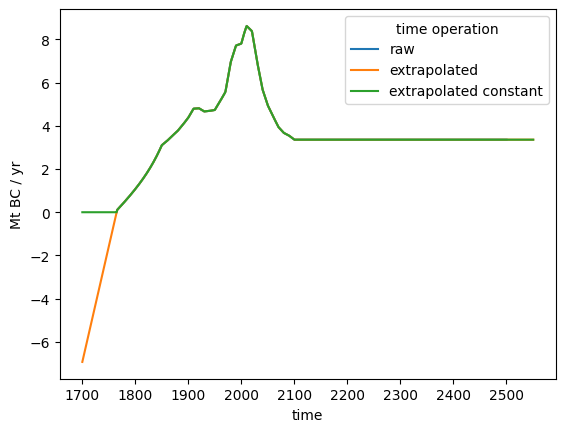
../_images/cba4509cf3d3b6f49bf68fa4200e1c987744cb39c522d809cf2af320ed4ff359.png

If we try to extrapolate beyond our source data but set extrapolation_type=None, we will receive an InsufficientDataError.

try:
    rcp26.interpolate(
        target_times=sorted([dt.datetime(v, 7, 1) for v in range(1700, 2551)]),
        extrapolation_type=None,
    )
except scmdata.time.InsufficientDataError:
    traceback.print_exc(limit=0, chain=False)

scmdata.errors.InsufficientDataError: Target time points are outside the source time points, use an extrapolation type other than None

Generally the interpolate requires at minimum 3 times in order to perform any interpolation/extrapolation, otherwise an InsufficientDataError is raised. There is a special case where constant extrapolation can be used on a single time-step.

rcp26_yr2000 = rcp26.filter(year=2000)
rcp26_extrap_const_single = rcp26_yr2000.interpolate(
    target_times=sorted([dt.datetime(v, 7, 1) for v in range(1700, 2551)]),
    extrapolation_type="constant",
)
rcp26_extrap_const_single["time operation"] = "extrapolated constant"
rcp26_extrap_const_single.head()

					time	1700-07-01 00:00:00	1701-07-01 00:00:00	1702-07-01 00:00:00	1703-07-01 00:00:00	1704-07-01 00:00:00	1705-07-01 00:00:00	1706-07-01 00:00:00	1707-07-01 00:00:00	1708-07-01 00:00:00	1709-07-01 00:00:00	...	2541-07-01 00:00:00	2542-07-01 00:00:00	2543-07-01 00:00:00	2544-07-01 00:00:00	2545-07-01 00:00:00	2546-07-01 00:00:00	2547-07-01 00:00:00	2548-07-01 00:00:00	2549-07-01 00:00:00	2550-07-01 00:00:00
model	region	scenario	time operation	unit	variable
IMAGE	World	RCP26	extrapolated constant	Mt BC / yr	Emissions\|BC	7.8048	7.8048	7.8048	7.8048	7.8048	7.8048	7.8048	7.8048	7.8048	7.8048	...	7.8048	7.8048	7.8048	7.8048	7.8048	7.8048	7.8048	7.8048	7.8048	7.8048
				kt C2F6 / yr	Emissions\|C2F6	2.3749	2.3749	2.3749	2.3749	2.3749	2.3749	2.3749	2.3749	2.3749	2.3749	...	2.3749	2.3749	2.3749	2.3749	2.3749	2.3749	2.3749	2.3749	2.3749	2.3749
				kt C6F14 / yr	Emissions\|C6F14	0.4624	0.4624	0.4624	0.4624	0.4624	0.4624	0.4624	0.4624	0.4624	0.4624	...	0.4624	0.4624	0.4624	0.4624	0.4624	0.4624	0.4624	0.4624	0.4624	0.4624
				kt CCl4 / yr	Emissions\|CCl4	74.1320	74.1320	74.1320	74.1320	74.1320	74.1320	74.1320	74.1320	74.1320	74.1320	...	74.1320	74.1320	74.1320	74.1320	74.1320	74.1320	74.1320	74.1320	74.1320	74.1320
				kt CF4 / yr	Emissions\|CF4	12.0001	12.0001	12.0001	12.0001	12.0001	12.0001	12.0001	12.0001	12.0001	12.0001	...	12.0001	12.0001	12.0001	12.0001	12.0001	12.0001	12.0001	12.0001	12.0001	12.0001

5 rows × 851 columns

Time means

With monthly data, we can then take time means. Most of the time we just want to take the annual mean. This can be done as shown below.

Annual mean

rcp26_annual_mean = rcp26_monthly.time_mean("AC")
rcp26_annual_mean["time operation"] = "annual mean"
rcp26_annual_mean.head()

					time	1765-07-01 00:00:00	1766-07-01 00:00:00	1767-07-01 00:00:00	1768-07-01 00:00:00	1769-07-01 00:00:00	1770-07-01 00:00:00	1771-07-01 00:00:00	1772-07-01 00:00:00	1773-07-01 00:00:00	1774-07-01 00:00:00	...	2491-07-01 00:00:00	2492-07-01 00:00:00	2493-07-01 00:00:00	2494-07-01 00:00:00	2495-07-01 00:00:00	2496-07-01 00:00:00	2497-07-01 00:00:00	2498-07-01 00:00:00	2499-07-01 00:00:00	2500-07-01 00:00:00
model	region	scenario	time operation	unit	variable
IMAGE	World	RCP26	annual mean	Mt BC / yr	Emissions\|BC	0.035676	0.111128	0.139999	0.166494	0.193071	0.219724	0.246444	0.273286	0.300220	0.327241	...	3.3578	3.3578	3.3578	3.3578	3.3578	3.3578	3.3578	3.3578	3.3578	3.3578
				kt C2F6 / yr	Emissions\|C2F6	0.000000	0.000000	0.000000	0.000000	0.000000	0.000000	0.000000	0.000000	0.000000	0.000000	...	0.0857	0.0857	0.0857	0.0857	0.0857	0.0857	0.0857	0.0857	0.0857	0.0857
				kt C6F14 / yr	Emissions\|C6F14	0.000000	0.000000	0.000000	0.000000	0.000000	0.000000	0.000000	0.000000	0.000000	0.000000	...	0.0887	0.0887	0.0887	0.0887	0.0887	0.0887	0.0887	0.0887	0.0887	0.0887
				kt CCl4 / yr	Emissions\|CCl4	0.000000	0.000000	0.000000	0.000000	0.000000	0.000000	0.000000	0.000000	0.000000	0.000000	...	0.0000	0.0000	0.0000	0.0000	0.0000	0.0000	0.0000	0.0000	0.0000	0.0000
				kt CF4 / yr	Emissions\|CF4	0.010759	0.010751	0.010747	0.010743	0.010739	0.010735	0.010730	0.010726	0.010722	0.010718	...	1.0920	1.0920	1.0920	1.0920	1.0920	1.0920	1.0920	1.0920	1.0920	1.0920

5 rows × 736 columns

As the data is an annual mean, we put it in July 1st (which is more or less the centre of the year).

Annual mean centred on January 1st

Sometimes we want to take annual means centred on January 1st, rather than the middle of the year. This can be done as shown.

rcp26_annual_mean_jan_1 = rcp26_monthly.time_mean("AS")
rcp26_annual_mean_jan_1["time operation"] = "annual mean Jan 1"
rcp26_annual_mean_jan_1.head()

					time	1765-01-01 00:00:00	1766-01-01 00:00:00	1767-01-01 00:00:00	1768-01-01 00:00:00	1769-01-01 00:00:00	1770-01-01 00:00:00	1771-01-01 00:00:00	1772-01-01 00:00:00	1773-01-01 00:00:00	1774-01-01 00:00:00	...	2491-01-01 00:00:00	2492-01-01 00:00:00	2493-01-01 00:00:00	2494-01-01 00:00:00	2495-01-01 00:00:00	2496-01-01 00:00:00	2497-01-01 00:00:00	2498-01-01 00:00:00	2499-01-01 00:00:00	2500-01-01 00:00:00
model	region	scenario	time operation	unit	variable
IMAGE	World	RCP26	annual mean Jan 1	Mt BC / yr	Emissions\|BC	0.008794	0.077819	0.126805	0.153223	0.179777	0.206387	0.233081	0.259840	0.286746	0.313719	...	3.3578	3.3578	3.3578	3.3578	3.3578	3.3578	3.3578	3.3578	3.3578	3.3578
				kt C2F6 / yr	Emissions\|C2F6	0.000000	0.000000	0.000000	0.000000	0.000000	0.000000	0.000000	0.000000	0.000000	0.000000	...	0.0857	0.0857	0.0857	0.0857	0.0857	0.0857	0.0857	0.0857	0.0857	0.0857
				kt C6F14 / yr	Emissions\|C6F14	0.000000	0.000000	0.000000	0.000000	0.000000	0.000000	0.000000	0.000000	0.000000	0.000000	...	0.0887	0.0887	0.0887	0.0887	0.0887	0.0887	0.0887	0.0887	0.0887	0.0887
				kt CCl4 / yr	Emissions\|CCl4	0.000000	0.000000	0.000000	0.000000	0.000000	0.000000	0.000000	0.000000	0.000000	0.000000	...	0.0000	0.0000	0.0000	0.0000	0.0000	0.0000	0.0000	0.0000	0.0000	0.0000
				kt CF4 / yr	Emissions\|CF4	0.010762	0.010755	0.010749	0.010745	0.010741	0.010737	0.010732	0.010728	0.010724	0.010720	...	1.0920	1.0920	1.0920	1.0920	1.0920	1.0920	1.0920	1.0920	1.0920	1.0920

5 rows × 736 columns

As the data is centred on January 1st, we put it in January 1st.

Annual mean centred on December 31st

Sometimes we want to take annual means centred on December 31st, rather than the middle of the year. This can be done as shown.

rcp26_annual_mean_dec_31 = rcp26_monthly.time_mean("A")
rcp26_annual_mean_dec_31["time operation"] = "annual mean Dec 31"
rcp26_annual_mean_dec_31.head()

					time	1764-12-31 00:00:00	1765-12-31 00:00:00	1766-12-31 00:00:00	1767-12-31 00:00:00	1768-12-31 00:00:00	1769-12-31 00:00:00	1770-12-31 00:00:00	1771-12-31 00:00:00	1772-12-31 00:00:00	1773-12-31 00:00:00	...	2490-12-31 00:00:00	2491-12-31 00:00:00	2492-12-31 00:00:00	2493-12-31 00:00:00	2494-12-31 00:00:00	2495-12-31 00:00:00	2496-12-31 00:00:00	2497-12-31 00:00:00	2498-12-31 00:00:00	2499-12-31 00:00:00
model	region	scenario	time operation	unit	variable
IMAGE	World	RCP26	annual mean Dec 31	Mt BC / yr	Emissions\|BC	0.008794	0.077819	0.126805	0.153223	0.179777	0.206387	0.233081	0.259840	0.286746	0.313719	...	3.3578	3.3578	3.3578	3.3578	3.3578	3.3578	3.3578	3.3578	3.3578	3.3578
				kt C2F6 / yr	Emissions\|C2F6	0.000000	0.000000	0.000000	0.000000	0.000000	0.000000	0.000000	0.000000	0.000000	0.000000	...	0.0857	0.0857	0.0857	0.0857	0.0857	0.0857	0.0857	0.0857	0.0857	0.0857
				kt C6F14 / yr	Emissions\|C6F14	0.000000	0.000000	0.000000	0.000000	0.000000	0.000000	0.000000	0.000000	0.000000	0.000000	...	0.0887	0.0887	0.0887	0.0887	0.0887	0.0887	0.0887	0.0887	0.0887	0.0887
				kt CCl4 / yr	Emissions\|CCl4	0.000000	0.000000	0.000000	0.000000	0.000000	0.000000	0.000000	0.000000	0.000000	0.000000	...	0.0000	0.0000	0.0000	0.0000	0.0000	0.0000	0.0000	0.0000	0.0000	0.0000
				kt CF4 / yr	Emissions\|CF4	0.010762	0.010755	0.010749	0.010745	0.010741	0.010737	0.010732	0.010728	0.010724	0.010720	...	1.0920	1.0920	1.0920	1.0920	1.0920	1.0920	1.0920	1.0920	1.0920	1.0920

5 rows × 736 columns

As the data is centred on December 31st, we put it in December 31st.

Comparing the results

We can compare the impact of these different methods with a plot as shown below.

var_to_plot = "Emissions|CF4"
pdf = run_append(
    [
        rcp26,
        rcp26_monthly,
        rcp26_start_of_year,
        rcp26_middle_of_year,
        rcp26_end_of_year,
        rcp26_annual_mean,
        rcp26_annual_mean_jan_1,
        rcp26_annual_mean_dec_31,
    ]
)

fig = plt.figure(figsize=(16, 9))

ax = fig.add_subplot(121)
pdf.filter(variable=var_to_plot).lineplot(ax=ax, hue="time operation")

ax = fig.add_subplot(122)
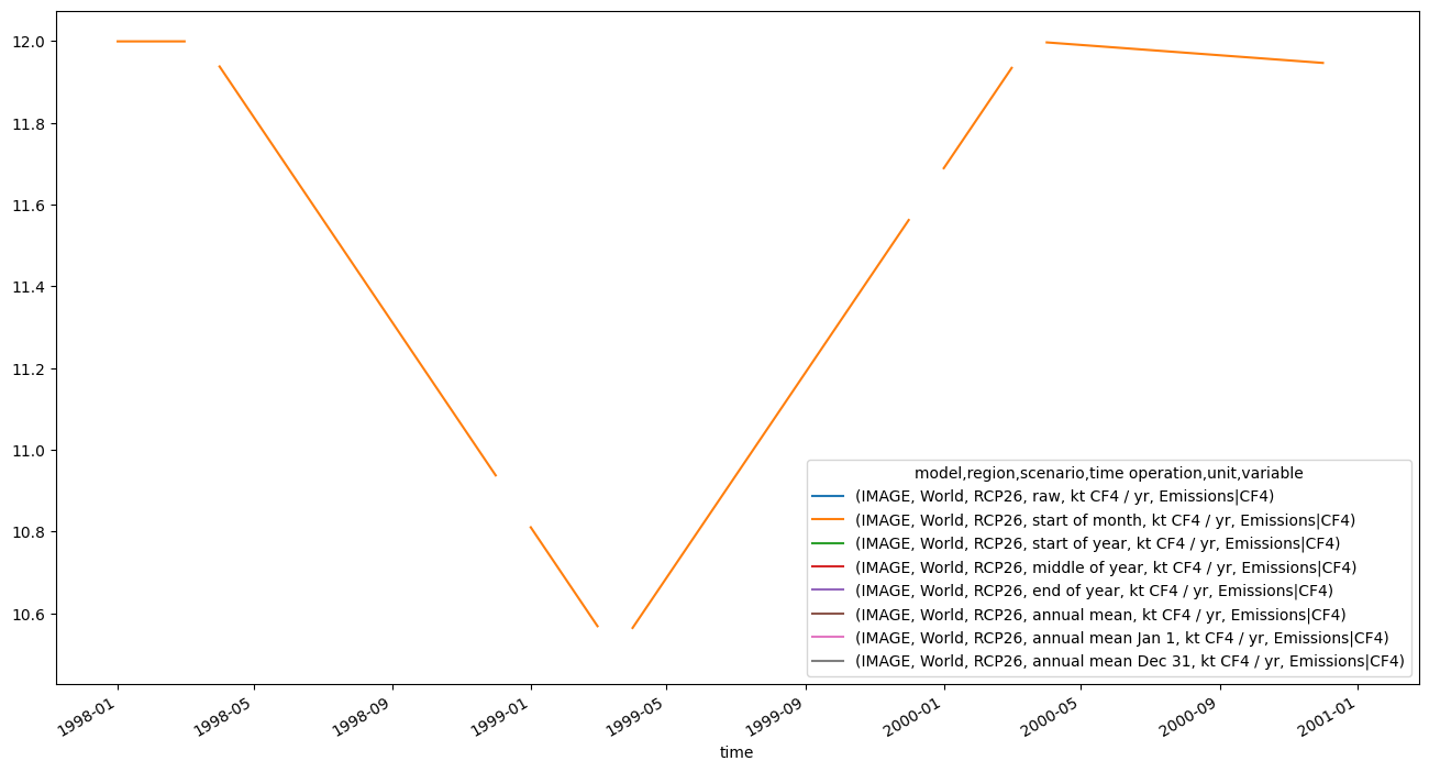
pdf.filter(variable=var_to_plot, year=range(1998, 2001)).lineplot(
    ax=ax, hue="time operation"
)

plt.tight_layout()

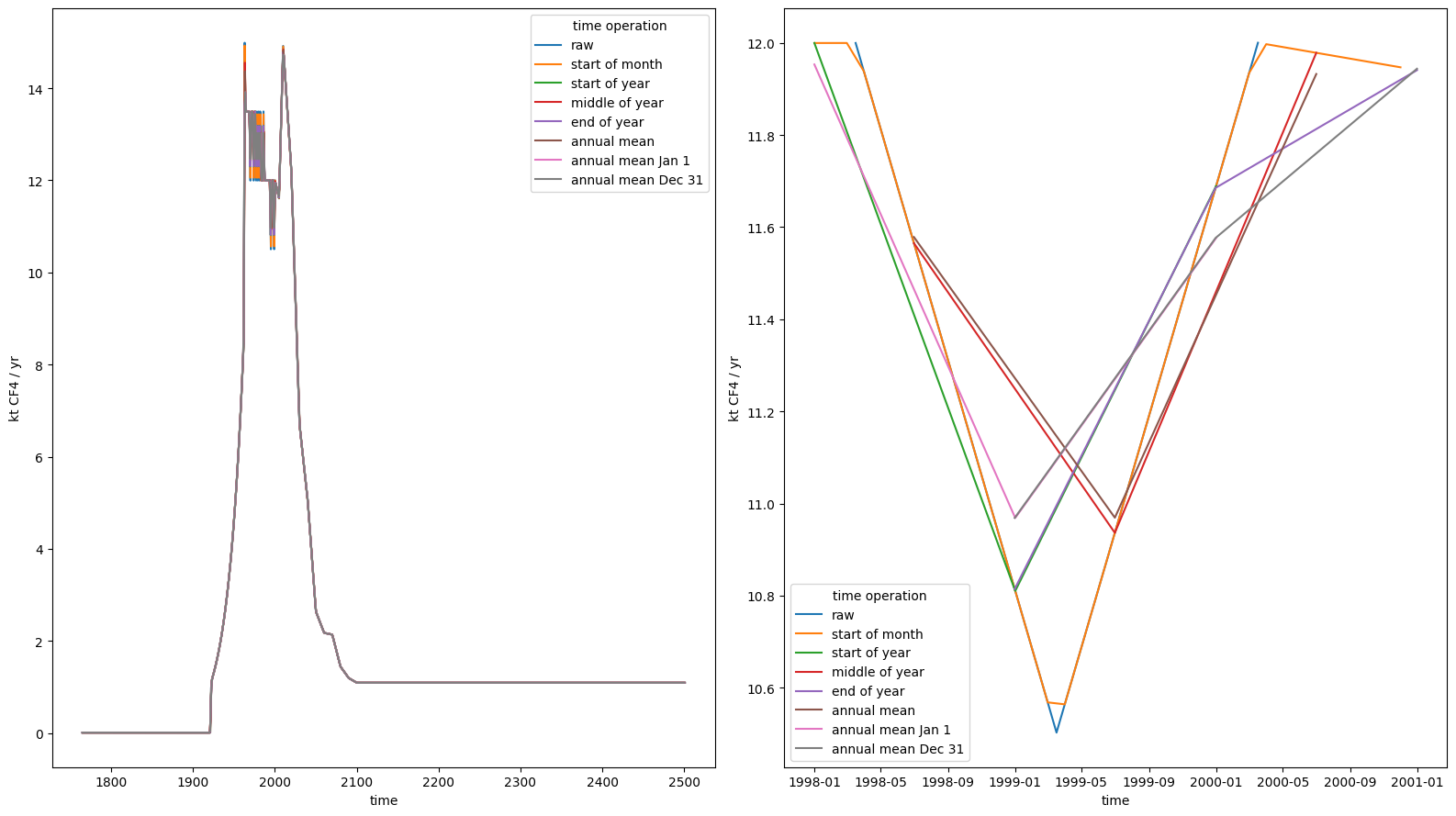
../_images/5629e68bd96cd903edc80cb89a32daf465b8690a05af70682a0c267403413be8.png

When the timeseries is particularly noisy, the different operations result in slightly different timeseries. For example, shifting to start of month smooths the data a bit (as you’re interpolating and resampling the underlying data) while taking means centred on different points in time changes your mean as you take different windows of your monthly data.

fig = plt.figure(figsize=(16, 9))

ax = fig.add_subplot(121)
pdf.filter(variable=var_to_plot).lineplot(ax=ax, hue="time operation")

ax = fig.add_subplot(122)
pdf.filter(variable=var_to_plot, year=range(1998, 2001)).lineplot(
    ax=ax, hue="time operation", legend=False
)

plt.tight_layout()

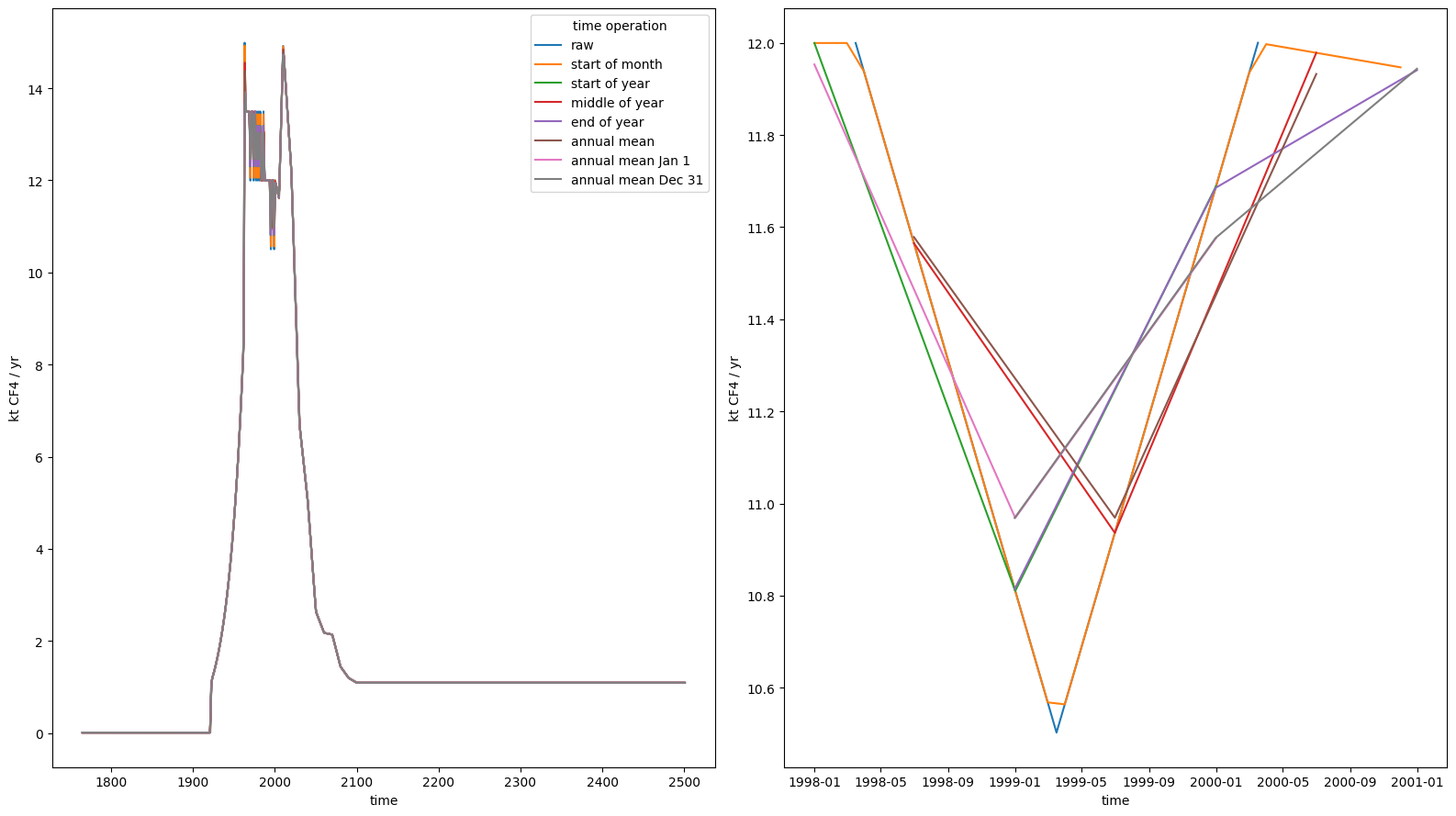
../_images/5b33329c071879d18cb98e4b471e85bec3ef1576ca62727a118448f1766fc6ee.png

The lines above don’t match the underlying timeseries e.g. the monthly data minimum is in the wrong place.

rcp26_monthly.filter(
    variable=var_to_plot, year=range(1998, 2001), month=[2, 3, 4, 5]
).timeseries()

					time	1998-02-01	1998-03-01	1998-04-01	1998-05-01	1999-02-01	1999-03-01	1999-04-01	1999-05-01	2000-02-01	2000-03-01	2000-04-01	2000-05-01
model	region	scenario	time operation	unit	variable
IMAGE	World	RCP26	start of month	kt CF4 / yr	Emissions\|CF4	11.999545	11.999564	11.938059	11.815028	10.683138	10.568309	10.564061	10.6868	11.815992	11.93464	11.997014	11.990841

pdf.filter(variable=var_to_plot, year=range(1998, 2001)).timeseries().T.plot(
    figsize=(16, 9)
)

<Axes: xlabel='time'>

../_images/d44fcb950da1c4d27b6d3b6d00e574996d1c67ebf0f16597ee6bd7beae83aa7c.png

pdf.filter(variable=var_to_plot, year=range(1998, 2001)).timeseries().T.sort_index()

model	IMAGE
region	World
scenario	RCP26
time operation	raw	start of month	start of year	middle of year	end of year	annual mean	annual mean Jan 1	annual mean Dec 31
unit	kt CF4 / yr	kt CF4 / yr	kt CF4 / yr	kt CF4 / yr	kt CF4 / yr	kt CF4 / yr	kt CF4 / yr	kt CF4 / yr
variable	Emissions\|CF4	Emissions\|CF4	Emissions\|CF4	Emissions\|CF4	Emissions\|CF4	Emissions\|CF4	Emissions\|CF4	Emissions\|CF4
time
1998-01-01	NaN	11.999523	11.999523	NaN	NaN	NaN	11.953026	NaN
1998-02-01	NaN	11.999545	NaN	NaN	NaN	NaN	NaN	NaN
1998-03-01	NaN	11.999564	NaN	NaN	NaN	NaN	NaN	NaN
1998-03-17	11.999575	NaN	NaN	NaN	NaN	NaN	NaN	NaN
1998-04-01	NaN	11.938059	NaN	NaN	NaN	NaN	NaN	NaN
1998-05-01	NaN	11.815028	NaN	NaN	NaN	NaN	NaN	NaN
1998-06-01	NaN	11.687895	NaN	NaN	NaN	NaN	NaN	NaN
1998-07-01	NaN	11.564864	NaN	11.564864	NaN	11.578184	NaN	NaN
1998-08-01	NaN	11.437731	NaN	NaN	NaN	NaN	NaN	NaN
1998-09-01	NaN	11.310599	NaN	NaN	NaN	NaN	NaN	NaN
1998-10-01	NaN	11.187567	NaN	NaN	NaN	NaN	NaN	NaN
1998-11-01	NaN	11.060435	NaN	NaN	NaN	NaN	NaN	NaN
1998-12-01	NaN	10.937403	NaN	NaN	NaN	NaN	NaN	NaN
1998-12-31	NaN	NaN	NaN	NaN	10.814372	NaN	NaN	10.968734
1999-01-01	NaN	10.810271	10.810271	NaN	NaN	NaN	10.968734	NaN
1999-02-01	NaN	10.683138	NaN	NaN	NaN	NaN	NaN	NaN
1999-03-01	NaN	10.568309	NaN	NaN	NaN	NaN	NaN	NaN
1999-03-17	10.502692	NaN	NaN	NaN	NaN	NaN	NaN	NaN
1999-04-01	NaN	10.564061	NaN	NaN	NaN	NaN	NaN	NaN
1999-05-01	NaN	10.686800	NaN	NaN	NaN	NaN	NaN	NaN
1999-06-01	NaN	10.813629	NaN	NaN	NaN	NaN	NaN	NaN
1999-07-01	NaN	10.936368	NaN	10.936368	NaN	10.969208	NaN	NaN
1999-08-01	NaN	11.063197	NaN	NaN	NaN	NaN	NaN	NaN
1999-09-01	NaN	11.190027	NaN	NaN	NaN	NaN	NaN	NaN
1999-10-01	NaN	11.312765	NaN	NaN	NaN	NaN	NaN	NaN
1999-11-01	NaN	11.439595	NaN	NaN	NaN	NaN	NaN	NaN
1999-12-01	NaN	11.562333	NaN	NaN	NaN	NaN	NaN	NaN
1999-12-31	NaN	NaN	NaN	NaN	11.685072	NaN	NaN	11.576366
2000-01-01	NaN	11.689163	11.689163	NaN	NaN	NaN	11.576366	NaN
2000-02-01	NaN	11.815992	NaN	NaN	NaN	NaN	NaN	NaN
2000-03-01	NaN	11.934640	NaN	NaN	NaN	NaN	NaN	NaN
2000-03-17	12.000100	NaN	NaN	NaN	NaN	NaN	NaN	NaN
2000-04-01	NaN	11.997014	NaN	NaN	NaN	NaN	NaN	NaN
2000-05-01	NaN	11.990841	NaN	NaN	NaN	NaN	NaN	NaN
2000-06-01	NaN	11.984463	NaN	NaN	NaN	NaN	NaN	NaN
2000-07-01	NaN	11.978290	NaN	11.978290	NaN	11.932250	NaN	NaN
2000-08-01	NaN	11.971912	NaN	NaN	NaN	NaN	NaN	NaN
2000-09-01	NaN	11.965533	NaN	NaN	NaN	NaN	NaN	NaN
2000-10-01	NaN	11.959361	NaN	NaN	NaN	NaN	NaN	NaN
2000-11-01	NaN	11.952982	NaN	NaN	NaN	NaN	NaN	NaN
2000-12-01	NaN	11.946810	NaN	NaN	NaN	NaN	NaN	NaN
2000-12-31	NaN	NaN	NaN	NaN	11.940637	NaN	NaN	11.943668